Introduction to Linear Regression Analysis: How to do Linear Regression Analysis in R in Six Steps

Contents hide

1 Step 1: Make Sure Linear Regression is Appropriate for your Problem

1.1 Clustered Data

1.2 Data with Complex Non-Linearities

1.3 Temporal Data

1.4 Data where the response variable is not continuous

2 Step 2: Partition your data for model selection (train) and inference (test)

3 Step 3: Check assumptions on your model selection data

4 Step 4: Fix Assumption Violations

5 Step 5: Check Assumptions of Model Fit

6 Step 6: Analyze Model Fit and Interpret linear regression parameters

In this article we describe how to perform linear regression. We go over some linear regression basics and answer the question ‘how does linear regression work?’ from a practical standpoint. We focus on inference rather than prediction. However, much of what we’re saying applies to prediction as well.

Step 1: Make Sure Linear Regression is Appropriate for your Problem

Before seeing features and responses and saying, ‘let’s try linear regression,’ ask ‘should I use standard linear regression?’ Here, we describe cases where naively applying linear regression isn’t appropriate.

Clustered Data

One shouldn’t use the standard linear model for data that is clustered into groups. For instance, if we have features and responses from patients but patients are grouped by doctor or hospital. The effect of the covariates for a patient on a response will vary by the doctor or hospital, causing violations of the uncorrelated errors assumption. One can use linear mixed models to deal with this.

Data with Complex Non-Linearities

We can model complex non-linearities via data transformations, but at some point the resulting model becomes uninterpretable. Alternatively, one can summarize the raw data: either the features or responses. For instance, one can turn a continuous-valued $y$ or some feature into levels. This allows one to avoid fully describing the non-linearity and makes interpretation easier. However, changing $y$ this way may cause violations of the assumption that $y|X$ is Gaussian. One can handle this is via generalized linear models (GLMs).

Temporal Data

For data ordered in time, fitting linear regression naively often leads to serial correlation. This violates uncorrelated errors. One should use time series models to deal with this.

Data where the response variable is not continuous

As mentioned in the non-linearities section, often the response value is not continuous: it may be count data, binary, or ordinal. In this case given that $y|X$ is not Gaussian, we’d like to make a different assumption about its distribution. For count data this is often Poisson, for binary often logistic, and for ordinal data one uses several logistic distributions. The standard linear regression model is rarely appropriate.

Step 2: Partition your data for model selection (train) and inference (test)

In predictive modeling/machine learning one learns to divide data into train and test. Hypothesis testing requires something similar. Doing inference on a dataset, then looking for violations, correcting them, and doing inference on the same dataset is cheating. One needs to partition one’s data for model selection and inference. Unlike in predictive modeling/machine learning where one generally takes a large training dataset and a small test dataset, for model selection often one can use a minority of the dataset to discover and fix the major violations, and then test on the majority of the dataset: this helps because larger samples help both achieve significance, and allow the central limit theorem to be invoked when normality assumptions are violated.

Let’s get started by loading a dataset in R and partitioning it into train (model selection) and test (inference).

library(mlbench)
data(BostonHousing)
train=BostonHousing[1:100,]
test=BostonHousing[101:nrow(BostonHousing),]

Step 3: Check assumptions on your model selection data

We now need to check assumptions on the data set aside for model selection. There are five major ones:

Linearity
Homoskedasticity
Uncorrelated errors
Gaussian errors
No perfect multicollinearity, low multicollinearity

For more detail on how to check these assumptions, see here. We will do a very basic pass now.

Let’s fit the following model on the training data

plot(lm(medv ~ crim + rm + tax + lstat , data = train))

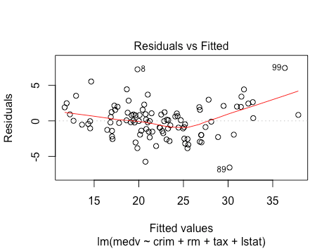
It looks like there is some non-linearity from the residuals vs. fitted plot. It’s difficult to determine whether there is heteroskedasticity or not.

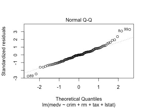
The qq-plot suggests some right skewness. Hard to tell on the left side.

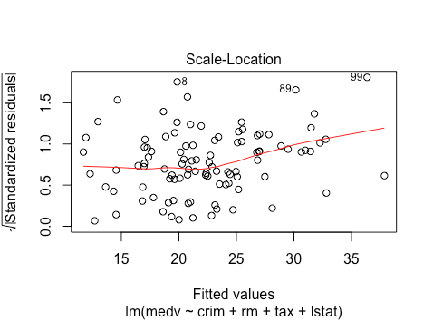
The scale location plot suggests some non-linearity as well as a bit of heteroskedasticity, since the mean magnitude is changing.

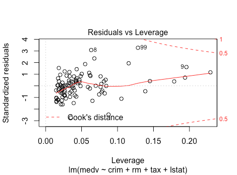
The residuals vs. leverage looks good. No clear outliers.

Step 4: Fix Assumption Violations

We generally apply transformations to fix assumption violations: we can transform either features or response. While transforming them to handle non-linearity is intuitive, we can also transform variables to correct for non-Gaussian residuals or heteroskedasticity. Choosing appropriate transformations is probably the trickiest part of using linear regression. For some description of log transformations, see here and here. Let’s try log-transforming the response for this model.

plot(lm(log(medv) ~ crim + rm + tax + lstat , data = train))

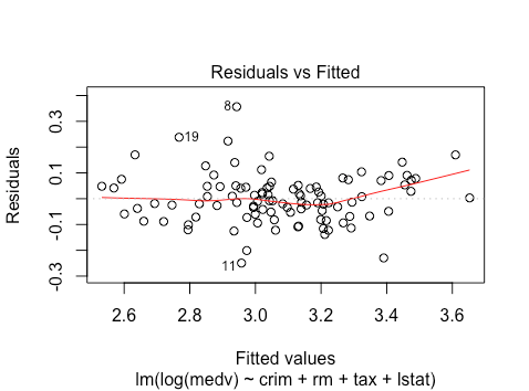
We see that the linearity issues seem to be reduced, although there is still a bit of non-linearity.

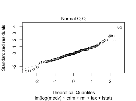
The qq-plot looks about the same. However, with >400 observations in the final test dataset, we can likely invoke the central limit theorem.

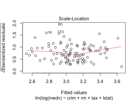
The scale location plot looks much better/more linear: this suggests a reduction in heteroskedasticity.

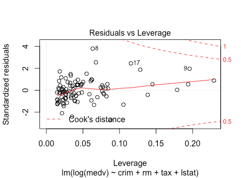
The residuals vs. leverage still doesn’t show any outliers. In sum, for training purposes at least, a log-transformation looks good. Let’s see what the resulting model says about coefficients. Note that because we did a transformation after fitting a model, we can’t take the resulting test statistics seriously. However, they can inform model selection that we will use on the test data.

summary(lm(log(medv) ~ crim + rm + tax + lstat , data = train))

 Call:
 lm(formula = log(medv) ~ crim + rm + tax + lstat, data = train)
 Residuals:
      Min       1Q   Median       3Q      Max 
 -0.24955 -0.05945 -0.00921  0.04820  0.35666 
 Coefficients:
               Estimate Std. Error t value Pr(>|t|)    
 (Intercept)  1.9198737  0.1977515   9.709 6.93e-16 ***
 crim        -0.1822366  0.0302235  -6.030 3.13e-08 ***
 rm           0.2414320  0.0256460   9.414 2.96e-15 ***
 tax         -0.0004638  0.0002232  -2.078   0.0404 *  
 lstat       -0.0154842  0.0024286  -6.376 6.54e-09 ***
 Signif. codes:  0 ‘’ 0.001 ‘’ 0.01 ‘’ 0.05 ‘.’ 0.1 ‘ ’ 1
 Residual standard error: 0.09693 on 95 degrees of freedom
 Multiple R-squared:  0.8609,    Adjusted R-squared:  0.8551 
 F-statistic:   147 on 4 and 95 DF,  p-value: < 2.2e-16

It appears that all coefficients are ‘significant.’ That suggests that we should use them in our final model.

Step 5: Check Assumptions of Model Fit

Now let’s move to the test data. We again have to look at the plots and hope that the assumptions are still met.

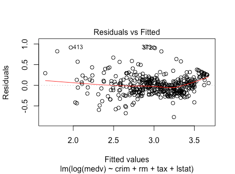
As we can see, there seems to be a bit more non-linearity here. There may also be heteroskedasticity. It seems that the spread of residuals for fitted values >3.5 is smaller.

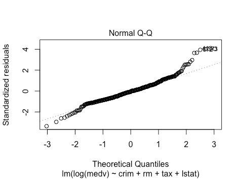
The normality assumption violations are also worse. However, we likely have enough data (>400 observations) to invoke the central limit theorem.

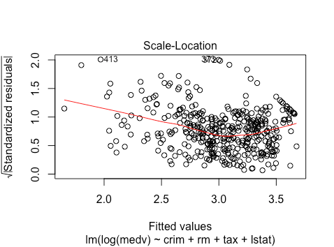
Again, non-linearity issues, and more heteroskedasticity.

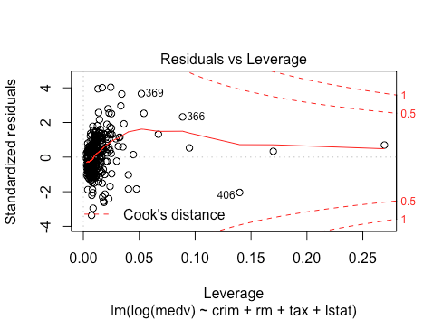
No outliers still. Overall, the violations seem to be worse on the testing data. Since this is testing data, we cannot make further changes to the model on the same data, and have to take it as given. The violations imply that we have to be a bit more suspicious of the resulting p-values and coefficients. Since the violations are not terrible, we can still use the resulting model fit and hypothesis tests.

Step 6: Analyze Model Fit and Interpret linear regression parameters

We now look at the resulting fit along with test statistics.

summary(lm(log(medv) ~ crim + rm + tax + lstat , data = test))

 Call:
 lm(formula = log(medv) ~ crim + rm + tax + lstat, data = test)
 Residuals:
      Min       1Q   Median       3Q      Max 
 -0.76991 -0.14897 -0.01448  0.11731  0.91516 
 Coefficients:
               Estimate Std. Error t value Pr(>|t|)    
 (Intercept)  2.855e+00  1.449e-01  19.701  < 2e-16 ***
 crim        -8.255e-03  1.509e-03  -5.471 7.92e-08 ***
 rm           1.205e-01  1.972e-02   6.111 2.35e-09 ***
 tax         -3.325e-04  8.709e-05  -3.819 0.000156 ***
 lstat       -3.104e-02  2.334e-03 -13.302  < 2e-16 ***
 Signif. codes:  0 ‘’ 0.001 ‘’ 0.01 ‘’ 0.05 ‘.’ 0.1 ‘ ’ 1
 Residual standard error: 0.2299 on 401 degrees of freedom
 Multiple R-squared:  0.7276,    Adjusted R-squared:  0.7249 
 F-statistic: 267.8 on 4 and 401 DF,  p-value: < 2.2e-16

We again see that all of our coefficients are individually significant, as is our intercept. The $R^2$ is pretty good: our model explains $73\%$ of the variation in the response. Unsurprisingly the F-test also tells us that the vector of coefficients is also significantly different from $0$ .

How do we interpret parameters here? Firstly note that they initially appear small. However, recall that we did a log transformation of the response. This changes the interpretation. In particular say we have a feature $x_1$ with coefficient $\beta_1$ , which is positive. The feature $x_1$ now has a multiplicative effect. A unit increase in $x_1$ leads to an expected increase of $y$ by a factor of $\exp(\beta_1)$ . Alternatively, a unit increase in $x_1$ leads to an increase of $y$ by $(\exp(\beta_1)-1)*100$ percent.

Look at rm, the number of rooms, with $\beta_2=0.1205$ . Then an increase in one room leads to an expected increase in price of of about $13\%$ . Note that with the analysis we did, this is an associative or predictive statement and not a causal one. We can’t use it to say that building another room will tend to increase price by $13\%$ .

In conclusion, in this post, we go over seven steps to go through when applying linear regression. Steps 3 and 4 should involve lots of trial and error, iteratively thinking about assumptions and trying different transformations and feature selection. Once one reaches step 5, trial and error needs to stop, and only analysis should be done.