Linear Regression: Comparing Models Between Two Groups with linearHypothesis

Contents hide

1 Without Regression: Testing Marginal Means Between Two Groups

2 Testing Conditional Means Between Two Groups

4 Testing The Differences Between the Two Groups in R

In this post, we describe how to compare linear regression models between two groups.

Without Regression: Testing Marginal Means Between Two Groups

In statistics, one often wants to test for a difference between two groups. A common setting involves testing for a difference in treatment effect. For instance, in a randomized trial experimenters may give drug A to one group and drug B to another, and then test for a statistically significant difference in the mean response of some biomarker (measurement) or outcome (ex: survival over some period) between the two groups. We generally want to test

(1) $\begin{align*}&H_0:\mathbb{E}[y_A]=\mathbb{E}[y_B]\\&H_1:\mathbb{E}[y_A]\neq\mathbb{E}[y_B]\end{align*}$

we are interested in whether $A$ and $B$ have the same mean response?

Testing Conditional Means Between Two Groups

While the marginal mean responses are interesting, often one cares about the distribution, conditioned on some covariates: so whether $\mathbb{E}[y_A|x]\overset{d}{=}\mathbb{E}[y_B|x]$ . That is: is there a difference between the groups, holding covariates, such as age, weight, or race fixed?

Let’s say we use linear regression to model both $\mathbb{E}[y_A|x]$ and $\mathbb{E}[y_B|x]$ . How can we test the following?

$H_0:\mathbb{E}[y_A|x]=\mathbb{E}[y_B|x]$
$H_0:\mathbb{E}[y_A|x]\neq\mathbb{E}[y_B|x]$

The key is to note that if we assume that our errors have mean $0$ and that our model specification is correct, then $\mathbb{E}[y|x]$ is completely determined by our parameters $\boldsymbol{\beta}$ . We can then include parameters that describe the difference between the two groups and test whether these parameters are significantly different from $0$ . The easiest way to do this is to repeat the same covariates as in an original model, but this time with interaction terms between those and some dummy (Indicator) variables representing which group one belongs to. So the original model would be:

$y_i=\beta_0+\beta_1 x_1^{(i)}+\cdots+\beta_p x_p^{(i)}+\epsilon_i,i=1,\cdots,n$

while the new model would use terms $I(A),I(B)$ , where

(2) $\begin{align*}I(A)&=\begin{cases}1\textrm{ group A}\\0\textrm{ group B}\end{cases}\end{align*}$

We would then use

(3) $\begin{align*}y_i&=\beta_0+\beta_{0,A}I(A)+\beta_{1,A} x_1^{(i)}I(A)\\&+\beta_{1,B} x_1^{(i)} I(B)+\cdots+\beta_{p,A}x_p^{(i)}I(A)\\&+\beta_{p,B} x_{p,B}^{(i)}I(B)+\epsilon_i\end{align*}$

Note that we use a single indicator for $\beta_0$ rather than one for each group because using one for each group would give us perfect multi-collinearity. We would then like to test

(4) $\begin{align*}&H_0:\beta_A=\beta_B\\&H_1:\beta_A\neq \beta_B\end{align*}$

Intuitively, we are asking: do groups A and B have different regression coefficients? We may also wish to exclude $\beta_{0,A}$ from this test in order to make sure that the null hypothesis only describes whether the covariates have a different effect across groups, rather than whether there is a different baseline across groups.

Real Data

Let’s try doing this on the Boston housing price dataset. We will test whether there is a difference in the effect of crime, tax rate, and lower status percent on median prices for areas with ‘big’ houses vs ‘small’ houses. Let’s load the data and make a histogram of the median # of rooms to see how to stratify into groups.

library(mlbench)
data(BostonHousing)
hist(BostonHousing[['rm']],main='Histogram of # of Rooms',xlab='# of Rooms')

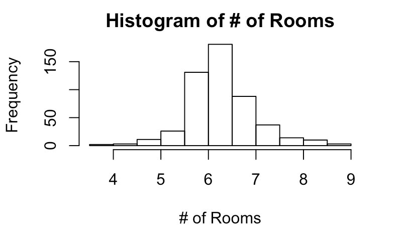
Based on this, it seems reasonable to stratify into two groups: median >6 rooms and <=6 rooms.

BostonHousing[['big']]<-as.numeric(BostonHousing[['rm']]>6)

We can then fit a model and look at the summary. Note that we will ignore checking model assumptions and the details of covariate/feature selection as we’re focused on comparing two groups.

fit<-lm(medv ~ big+I(crim*big)+I(crim*(1-big)) + I(tax *big)+I(tax*(1-big))+ I(lstat*(big))+I(lstat*(1-big)) , data = BostonHousing)
summary(fit)

Call:
lm(formula = medv ~ big + I(crim * big) + I(crim * (1 - big)) + 
    I(tax * big) + I(tax * (1 - big)) + I(lstat * (big)) + I(lstat * 
    (1 - big)), data = BostonHousing)

Residuals:
     Min       1Q   Median       3Q      Max 
-16.1621  -3.3619  -0.9198   2.0725  29.1939 

Coefficients:
                       Estimate Std. Error t value Pr(>|t|)    
(Intercept)          26.2100954  1.5522301  16.885  < 2e-16 ***
big                  11.6246444  1.8104137   6.421 3.16e-10 ***
I(crim * big)        -0.0124625  0.0610095  -0.204   0.8382    
I(crim * (1 - big))  -0.1188344  0.0490509  -2.423   0.0158 *  
I(tax * big)         -0.0004341  0.0028769  -0.151   0.8801    
I(tax * (1 - big))   -0.0007021  0.0031429  -0.223   0.8233    
I(lstat * (big))     -1.2250688  0.0746558 -16.410  < 2e-16 ***
I(lstat * (1 - big)) -0.4452595  0.0677917  -6.568 1.29e-10 ***
---
Signif. codes:  0 ‘***’ 0.001 ‘**’ 0.01 ‘*’ 0.05 ‘.’ 0.1 ‘ ’ 1

Residual standard error: 5.771 on 498 degrees of freedom
Multiple R-squared:  0.6118,	Adjusted R-squared:  0.6063 
F-statistic: 112.1 on 7 and 498 DF,  p-value: < 2.2e-16

Note that big gives us whether it’s an area with ‘big’ houses and 1-big gives us whether it’s an area with ‘small’ houses. We can see that most coefficients look statistically significant, and see several interesting things:

the coefficient for the indicator variable big is fairly large compared to the intercept
crime has a weaker effect on price for big houses
taxes have similar effect on price across big and small houses
the percent of low status people has a stronger effect for big houses

Testing The Differences Between the Two Groups in R

Let’s do a formal test to see whether there is a statistically significant difference between the two groups: that is, is there a difference in the effects of crime, taxes, or percent low status between the groups? We can import the car package and use the linearHypothesis function to test this. To do this, we need to create a hypothesis matrix. Each row of the hypothesis will show the linear combination of covariates of our hypothesis, and our default is that this linear combination is equal to $0$ . Here we create this matrix.

row_1<-c(0,1,-1,0,0,0,0)
row_2<-c(0,0,0,1,-1,0,0)
row_3<-c(0,0,0,0,0,1,-1)
hypothesisMatrix <- matrix(rbind(row_1,row_2,row_3),nrow=3,ncol=7)

The first entry of every row corresponds to the intercept. Our null hypothesis is then that crime, tax, and percent low status have the same mean effect on price across the two groups.

Here the first, second, and third rows correspond to crime, tax, and percent low status, respectively. We can see the hypothesis test written out when we run the linearHypothesis function from the car package.

library(car)
linearHypothesis(fit,hypothesisMatrix)

Linear hypothesis test

Hypothesis:
I(crim * rm) - I(crim * (1 - rm)) = 0
I(tax * rm) - I(tax * (1 - rm)) = 0
I(lstat * (rm)) - I(lstat * (1 - rm)) = 0

Model 1: restricted model
Model 2: medv ~ I(crim * rm) + I(crim * (1 - rm)) + I(tax * rm) + I(tax * 
    (1 - rm)) + I(lstat * (rm)) + I(lstat * (1 - rm))

  Res.Df   RSS Df Sum of Sq      F    Pr(>F)    
1    502 19170                                  
2    499 15412  3    3758.7 40.567 < 2.2e-16 ***
---
Signif. codes:  0 ‘***’ 0.001 ‘**’ 0.01 ‘*’ 0.05 ‘.’ 0.1 ‘ ’ 1

Based on this, we reject the null hypothesis that the two models are the same in favor of the richer model that we proposed. Thus, we conclude that the effect of the covariates on price differs between the two groups.

Without Regression: Testing Marginal Means Between Two Groups

Testing Conditional Means Between Two Groups

Real Data

Testing The Differences Between the Two Groups in R

Related Posts

Leave a Reply Cancel reply