Kaplan Meier: Non-Parametric Survival Analysis in R

In this post we describe the Kaplan Meier non-parametric estimator of the survival function. We first describe what problem it solves, give a heuristic derivation, then go over its assumptions, go over confidence intervals and hypothesis testing, and then show how to plot a Kaplan Meier curve or curves. We conclude by comparing Kaplan Meier to Cox regression, describing why you would want to move from the Kaplan Meier model to the Cox model. These curves help visualize the survival distribution and compare survival functions across groups.

Problem Statement

To start with, we have a collection of death or event times of patients. We observe some patients, while others may be right censored. That is, we know that they lived up to a certain time, but don’t know what happened after. For censoring in clinical trials, this could be due to the study ending or them leaving the study. Often, we have only one simple variable with which we can stratify our patients, or none at all. We are interested in estimating the survival function

(1) $\begin{align*}S(t)&=P(T>t)\\&=1-F(t)\end{align*}$

here $T$ is a random variable representing the death or event time, and $F$ is the cumulative distribution function. If we have one simple covariate with which to stratify patients into groups, we’d like to estimate several survival functions, one for each group.

An important concept is the hazard, which completely defines the survival function. It describes the instantaneous risk of an event at time $t$ , conditional on survival up to time $t$ . It is given by

(2) $\begin{align*}\lambda(t)&=\lim_{dt\rightarrow 0}\frac{P(t\leq T\leq t+dt|T\geq t)}{dt}\end{align*}$

Based on the above, we have two goals. The first is estimating one or more survival functions: this is a density estimation problem. The second is comparing groups based on our variable or variables: are the survival functions the same across two groups? Specifically, are the hazards the same for all times up to study end time? Groups could be treatment groups, male/female, age groups, or income groups, to name a few. In order to handle this problem, we use a non-parametric estimator called the Kaplan-Meier estimator.

Intuition: How to Calculate the Kaplan Meier Survival Curve

The Kaplan Meier estimator or curve is a non-parametric frequency based estimator. Given $k$ fully observed event times, it assumes patients can only die at these fully observed event times $T_1<T_2<\cdots<T_k$ . We then make the frequency assumption that the probability of dying at $T_i$ , given survival up to $T_{i-1}$ , is the # of people who died at that time divided by the # at risk. That is, defining $T_0=0$ , $d_i$ the # of people who die at $T_i$ and $Y(T_i)$ the number at risk just before $T_i$ ,

(3) $\begin{align*}P(\textrm{die at }T_i|\textrm{survive until }T_{i-1})&=\frac{d_i}{Y(T_i)}\end{align*}$

This gives us the conditional survival function estimate

(4) $\begin{align*}\hat{S}(T_i|T_{i-1})&=1-\frac{d_i}{Y(T_i)}\end{align*}$

We then have

(5) $\begin{align*}\hat{S}(t)&=\prod_{T_i\leq t} \hat{S}(T_i|T_{i-1})\\&=\prod_{t_i\leq t} (1-\frac{d_i}{Y(T_i)})\end{align*}$

where the last line is the Kaplan-Meier estimator of the survival function. Essentially, it’s the product of probabilities of surviving at each candidate time, where each individual probability is $1$ minus a frequency-based death probability.

Assumptions of the Kaplan Meier estimator

The Kaplan Meier estimator makes two major assumptions in order to have good theoretical properties: independent censoring and iid data. Independent censoring means that the censoring distribution for an individual does not depend on their event time. How could this be violated? Let’s say as people get sicker, they tend to leave the study. However, sickness also increases death risk. This violates independent censoring: we call this informative dropout.

IID data is a standard assumption, but it’s worth thinking about how violations arise. In fact, any time there are important groupings that aren’t included in the model it is violated. For instance, say our patients have different ages, and age affects death risk, but it isn’t collected in our dataset. The true death risks will then cluster into age groups, making our data neither independent nor identically distributed.

Finally, in order to infer causal effects, we need a randomized stratification variable. For an unrandomized example, say male/female is our variable, and we’re modeling time to death for people with some disease. It’s possible that males receive treatment at a higher rate for this disease, and since male/female isn’t randomized by assignment we can’t say that being male caused the difference in survival probabilities. On the other hand, for treatment, we know from the study design whether it’s randomized, and if it is, we can conclude that difference in survival probabilities are treatment effects.

Kaplan Meier: Confidence Interval

Once we have our Kaplan Meier estimator, we can calculate confidence intervals using Greenwood’s formula for the standard error or variance.

(6) $\begin{align*}\tilde{\tau}^2(t)&=\hat{S}(t)^2\sum_{T_i\leq t}\frac{1}{Y(T_i)\{Y(T_i)-1\}}\\\tilde{\tau}(t)&=\hat{S}(t)\sqrt{\sum_{T_i\leq t}\frac{1}{Y(T_i)\{Y(T_i)-1\}}}\end{align*}$

We can also calculate a $100(1-\alpha)\%$ confidence interval

(7) $\begin{align*}\hat{S}(t)\pm z_{1-\alpha/2}\tilde{\tau}(t)\end{align*}$

Note that the intuition for this comes from continuous-time martingale theory and thus is beyond the scope of this article.

Log Rank Test: Kaplan Meier Hypothesis Testing

In order to test whether the survival functions are the same for two strata, we can test the null hypothesis

(8) $\begin{align*}H_0:\lambda_1(t)&=\lambda_2(t)\forall t\in [0,t_0]\\H_1:\lambda_1(t)&\neq\lambda_2(t)\forall t\in [0,t_0]\end{align*}$

we do so via the log rank test. Due to the use of continuous-time martingales, we will not go into detail on how this works. However, in the application section we describe the relevant R commands.

Kaplan Meier: Median and Mean Survival Times

In addition to the full survival function, we may also want to know median or mean survival times. To calculate the median is simple. Noting that our estimator is non-parametric and thus jumps at a finite set of points , we simply take $p=0.5$ and compute the smallest observed $T_i$ so that

(9) $\begin{align*}\hat{S}(t)&\leq 1-p\end{align*}$

For the mean, we can take

(10) $\begin{align*}\sum_{i=0}^{k-1}\hat{S}(T_i)(T_i-T_{i-1})\end{align*}$

however, survival times are not expected to be normally distributed, so in general the mean should not be computed as it is liable to be misinterpreted by those interpreting it.

Example: Kaplan Meier Cancer Application

Let’s now calculate the Kaplan Meier estimator for the ovarian cancer data in R. This has several variables:

futime: last observed time
fustat: censoring indicator
resid.ds: presence of residual disease
patient age
rx: treatment group assignment
ecog.ps: performance status, patient’s level of functioning in life

We start by loading the data

 library(survival)
 ovarian
    futime fustat     age resid.ds rx ecog.ps
 1      59      1 72.3315        2  1       1
 2     115      1 74.4932        2  1       1
 3     156      1 66.4658        2  1       2
 4     421      0 53.3644        2  2       1
 5     431      1 50.3397        2  1       1
 6     448      0 56.4301        1  1       2
 7     464      1 56.9370        2  2       2

Next we can fit Kaplan Meier, stratifying into two models based on treatment

#First setup survival object
km <- Surv(time = ovarian[['futime']], event = ovarian[['fustat']])
#Fit Kaplan Meier, stratifying by treatment
km_treatment<-survfit(km~rx,data=ovarian,type='kaplan-meier',conf.type='log')

#Print fit
km_treatment
Call: survfit(formula = km ~ rx, data = ovarian, type = "kaplan-meier", 
    conf.type = "log")

      n events median 0.95LCL 0.95UCL
rx=1 13      7    638     268      NA
rx=2 13      5     NA     475      NA

We see that in group $1$ , the median survival time is 638, while in group $2$ , there is no observed time leading to a probability greater than $0.5$ , and thus we cannot compute the median.

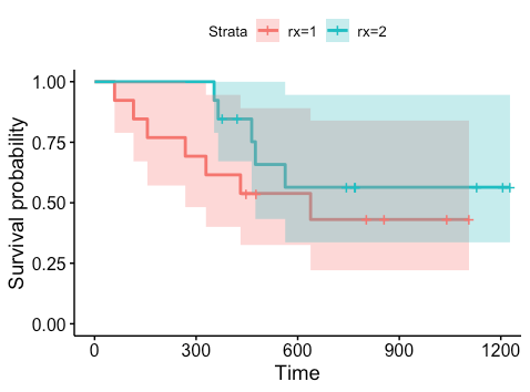
We can then plot the differences across the two groups. Using the default package makes somewhat ugly plots, so we instead use the survminer package.

library(survminer)
ggsurvplot(km_treatment,conf.int = 'True')

We can also conduct the hypothesis test described above.

survdiff(km~rx,data=ovarian)

 Call:
 survdiff(formula = km ~ rx, data = ovarian)
  N Observed Expected (O-E)^2/E (O-E)^2/V
 rx=1 13        7     5.23     0.596      1.06
 rx=2 13        5     6.77     0.461      1.06
 Chisq= 1.1  on 1 degrees of freedom, p= 0.3

As we can see we get a p-value of $0.3$ , and fail to reject the null hypothesis of a significant treatment effect.

Kaplan Meier vs Cox Proportional Hazards Model

Our analysis has one big problem: we assumed that within a treatment group we have iid patients, implying that we don’t have clustering by age, presence of residual disease, and performance status This seems unlikely. However, in order to incorporate these variables within a Kaplan Meier framework, we would need to stratify based on each variable. If we only take two groups per variable, this would lead to $2^4=16$ models! We only have 26 observations, so we can’t realistically do this.

One way to handle this is to assume that the effect of a change in one of these variables on the hazard is constant and multiplicative over time. This is the proportional hazards assumption. So for instance, if we stratify age into residual disease present and not present, present might have two times higher hazard at every possible time in the study. We can actually see in our Kaplan Meier plot above that this appears to not be the case for treatment, as if it was, the two groups would have the same high-level pattern but would diverge from each other. However, the sample size here is very small, so with more data, the proportional hazards assumption might hold (we simply don’t know due to lack of data).

With this intuition we can then move to a semi-parametric model: a flexible baseline hazard describes how the average person’s risk changes over time, while a parametric relative risk describes how covariates affect the risk. Click here to learn more about Cox regression.