Linear Regression: Log Transforming Response

There are several reasons to log transform the response. The obvious one is to fix linearity violations, but in many cases log transforming the response also reduces either heteroskedasticity or skewness of the residuals. In this post we show an ideal case for a log transformation of the dependent variable on synthetic data, then a case where it helps but doesn’t necessarily solve all problems.

Synthetic Data

Consider a case where we have the following as the true model

(1)  

Let’s create some synthetic data and fit the wrong model

   x1=runif(100,0,5)
   x2=runif(100,0,5)
   eps=rnorm(100,0,1)
   y=exp(2*x1+5*x2+eps)
   plot(lm(y~x1+x2))

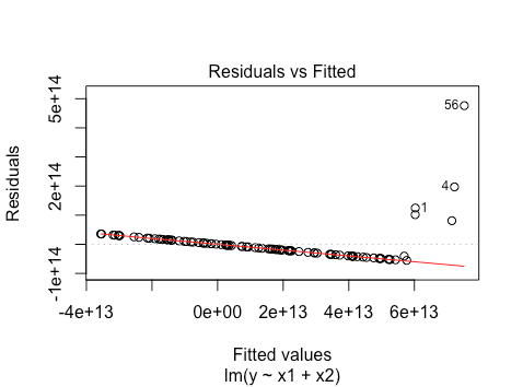
We want the residuals to be evenly spread around 0 for every fitted value. Here, the residuals have a strange pattern: most of them lie on a line that is decreasing and they have almost no spread except for at very large fitted values. However, if we apply a log transformation to the response, we see an improvement.

This looks exactly how it should, which makes sense as it uses a correctly specified model.

Real Data

In real data you rarely get such an extreme result from a transformation. Let’s see a case where a transformation helps somewhat with linearity, heteroskedasticity, and normality violations, but doesn’t fully fix any of them. We borrow some code from https://machinelearningmastery.com/machine-learning-datasets-in-r/ and https://www.kaggle.com/sukeshpabba/linear-regression-with-boston-housing-data.

library(mlbench)
data(BostonHousing)
plot(lm(medv ~ crim + rm + tax + lstat , data = BostonHousing))

There is some clear non-linearity here, as well as a bit of heteroskedasticity: for fitted values around 20 we see some much larger magnitude residuals. Let’s trying log-transforming the response.

plot(lm(log(medv) ~ crim + rm + tax + lstat , data = BostonHousing))

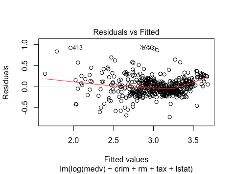
This improves the linearity, although only slightly. Further, it seems to decrease the heteroskedasticity, but again it’s still present. Let’s also look at the normality plots. For the untransformed response we have

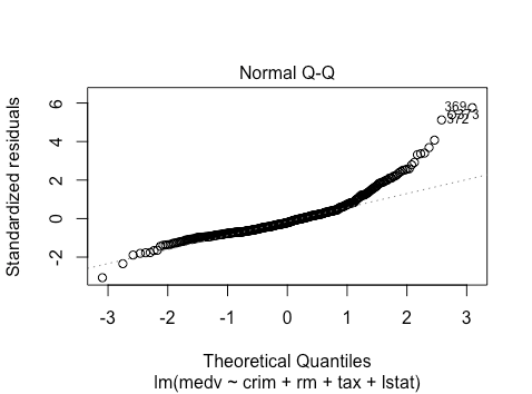
This is pretty bad. There is heavy skewness on the right. For the transformed response we have

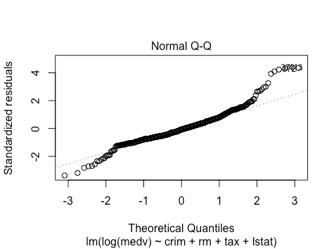
This exhibits less skewness on the right, but it is far from eliminated. This also now has a slightly fatter tail on the left than would be expected theoretically. Overall, the log transformation of the response has improved things somewhat, but not by enough to necessarily be confident about inferences.