In this post we check the assumptions of linear regression using Python. Linear regression models the relationship between a design matrix $\boldsymbol{X}$ of shape $n\times p$ ( $n$ observations and $p$ features) and a response vector $\boldsymbol{y}$ of length $n$ via the following equation:

(1) $\begin{align*}\boldsymbol{y}&=\boldsymbol{X}\beta+\boldsymbol{\epsilon}\end{align*}$

or for individual points $X^{(i)},y_i$

(2) $\begin{align*}y_i&=\beta^T X^{(i)}+\epsilon_i\end{align*}$

the $\epsilon_i$ are called the errors. We have five main assumptions for linear regression.

Linearity: there is a linear relationship between our features and responses. This is required for our estimator and predictions to be unbiased.
No multicollinearity: our features are not correlated. If this is not satisfied, our estimator will suffer from high variance.
Gaussian errors: our errors $\epsilon_i$ are Gaussian distributed with mean $0$ . This is necessary for a range of statistical tests, such as the t-test. We can relax this assumption in large samples due to the central limit theorem.
Homoskedasticity: our errors have equal variance. If this is not satisfied, there will be other linear estimators with lower variance.
Independent errors: our errors are independent. Violations can cause a wide range of problems for inference.

The last three assumptions can be summarized via the equation $\boldsymbol{\epsilon}\sim \mathcal{N}(0,\sigma^2 I)$ . Assumptions 1, 4, and a relaxation of 5 (uncorrelated errors) are needed for good predictions. Assumptions 2 and 3 are needed for good inferences.

We test the assumptions of linear regression on the kaggle dataset of housing prices https://www.kaggle.com/c/house-prices-advanced-regression-techniques/kernels. We start by importing required libraries.

#numerical libraries
import pandas as pd
import numpy as np
#plotting and visualization
import seaborn as sns
from matplotlib import pyplot as plt
import matplotlib
#statistical libraries from statsmodels.regression.linear_model import OLS import statsmodels as sm

We borrow some data pre-processing code from https://www.kaggle.com/apapiu/regularized-linear-models.

train = pd.read_csv("all/train.csv")
test = pd.read_csv("all/test.csv")
all_data = pd.concat((train.loc[:,'MSSubClass':'SaleCondition'],
                       test.loc[:,'MSSubClass':'SaleCondition']))
matplotlib.rcParams['figure.figsize'] = (12.0, 6.0)
prices = pd.DataFrame({"price":train["SalePrice"], "log(price + 1)":np.log1p(train["SalePrice"])})
all_data = pd.get_dummies(all_data)
#filling NA's with the mean of the column:
all_data = all_data.fillna(all_data.mean())
#creating relevant matrices:
X_train = all_data[:train.shape[0]]
X_test = all_data[train.shape[0]:]
y = train.SalePrice
X_train_np = np.array(X_train)
y_np = np.array(y)

Linearity

The first assumption we check is linearity. We can visually check this by fitting ordinary least squares (OLS) on some training data, and then using it to predict our training data. We then plot the predictions vs actual. We should observe that the points are approximately symmetric about a line through the origin with slope $1$ .

from scipy import stats
def abline(slope, intercept):
     """Plot a line from slope and intercept, borrowed from https://stackoverflow.com/questions/7941226/how-to-add-line-based-on-slope-and-intercept-in-matplotlib"""
     axes = plt.gca()
     x_vals = np.array(axes.get_xlim())
     y_vals = intercept + slope * x_vals
     plt.plot(x_vals, y_vals, '--')
 #fit an OLS model to data
 model = OLS(y_np,sm.tools.add_constant(X_train_np))
 results = model.fit()
 #predict y values for training data
 y_hat = model.predict(results.params)
 #plot predicted vs actual
 plt.plot(y_hat,y_np,'o')
 plt.xlabel('Predicted')#,color='white')
 plt.ylabel('Actual')#,color='white')
 plt.title('Predicted vs. Actual: Visual Linearity Test')#,color='white')
 plt.tick_params(axis='x', colors='white')
 plt.tick_params(axis='y', colors='white')
 abline(1,0)
 plt.show()

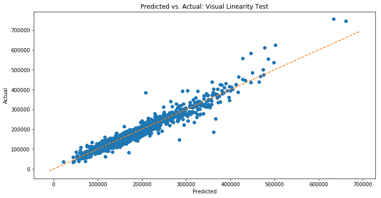
The plot looks pretty good! Violations of linearity aren’t obvious. We can then run (or maybe we can’t) a statistical test for linearity called Harvey Collier, which tests whether recursive residuals have mean $0$ (which they should under the null hypothesis of linearity). We will likely discuss both this test and recursive residuals in more detail in a future post.

from statsmodels.stats.diagnostic import linear_harvey_collier
print linear_harvey_collier(results)

--------------------------------------------------------------------------- LinAlgError                               Traceback (most recent call last) <ipython-input-16-4870b10cc03d> in <module>()       
1 from statsmodels.stats.diagnostic import linear_harvey_collier 
----> 2 print linear_harvey_collier(results) 
/anaconda2/lib/python2.7/site-packages/statsmodels/sandbox/stats/diagnostic.pyc in linear_harvey_collier(res)     
915     #B.H. Baltagi, Econometrics, 2011, chapter 8     
916     #but it matches Gretl and R:lmtest, pvalue at decimal=13 --> 917     rr = recursive_olsresiduals(res, skip=3, alpha=0.95)     
918     from scipy import stats     
919  /anaconda2/lib/python2.7/site-packages/statsmodels/sandbox/stats/diagnostic.pyc in recursive_olsresiduals(olsresults, skip, lamda, alpha)    
1172     y0 = y[:skip]    
1173     #add Ridge to start (not in jplv -> 1174     XTXi = np.linalg.inv(np.dot(x0.T, x0)+lamda*np.eye(nvars))    
1175     XTY = np.dot(x0.T, y0) #xi * y   #np.dot(xi, y)    
1176     #beta = np.linalg.solve(XTX, XTY) /anaconda2/lib/python2.7/site-packages/numpy/linalg/linalg.pyc in inv(a)     
526     signature = 'D->D' if isComplexType(t) else 'd->d'     
527     extobj = get_linalg_error_extobj(_raise_linalgerror_singular) 
--> 528     ainv = _umath_linalg.inv(a, signature=signature, extobj=extobj)     529     return wrap(ainv.astype(result_t, copy=False))     
530  /anaconda2/lib/python2.7/site-packages/numpy/linalg/linalg.pyc in _raise_linalgerror_singular(err, flag)      
87       
88 def _raise_linalgerror_singular(err, flag): 
---> 89     raise LinAlgError("Singular matrix")      
90       
91 def _raise_linalgerror_nonposdef(err, flag): LinAlgError: Singular matrix

We get an error! It mentions a singular matrix. This is very related to the next important assumption of linear regression.

Multicollinearity

Multicollinearity occurs when features are correlated: this causes our estimator to have high variance and thus be poor. We describe why this is a problem in more detail here. In order to detect multicollinearity, we use variance inflation factors (VIF). A VIF of over $10$ for some feature indicates that over $90\%$ of the variance in that feature is explained by the remaining features. Over $100$ indicates over $99\%$ .

from statsmodels.stats.outliers_influence import variance_inflation_factor
vif = [variance_inflation_factor(X_train_np, i) for i in range(X_train_np.shape[1])]
print vif


 /anaconda2/lib/python2.7/site-packages/statsmodels/stats/outliers_influence.py:181: RuntimeWarning: divide by zero encountered in double_scalars   vif = 1. / (1. - r_squared_i) 
  
 
 [34.956601736613386, 2.6789578302277746, 3.4100366640143416,
 5.61828312180688, 2.6892617768974247, 15.462690140722279, 3.7909400357313214,
 3.1217404387849514, inf, inf, inf, inf, inf, inf, inf, inf, 
3.0168223391797557, 1.4924175818273853, 4.1963265661836555, 3.177321051350987, 
3.543572615464872, 4.495423454897208, 6.911889661487289, 7.75740816482209, 
6.1838331924182945, 8.282721165617906, 8.149583070883184, 1.549897513320911, 
1.6796400311722999, 1.6623738302601956, 1.229190285241749, 1.387963992550775, 
237.1711330988761, 26.30853277082208, 1.2543397509602774, 1.3378435036663416, 
inf, inf, inf, inf, inf, inf, inf, 1.680289191777855, 1.7707630732654085, inf, 
inf, inf, inf, inf, inf, inf, inf, inf, inf, inf, inf, inf, inf, inf, inf, 
inf, inf, inf, inf, inf, inf, inf, inf, inf, inf, inf, inf, inf, inf, inf, 
inf, inf, inf, inf, inf, inf, inf, inf, inf, inf, inf, inf, inf, inf, inf, 
inf, inf, inf, inf, inf, inf, inf, inf, inf, inf, inf, inf, inf, inf, inf, 
inf, inf, inf, inf, inf, inf, inf, inf, inf, inf, inf, inf, inf, inf, inf, 
inf, inf, inf, inf, inf, inf, inf, inf, inf, inf, inf, inf, inf, inf, inf, 
inf, inf, inf, inf, inf, inf, inf, inf, inf, inf, inf, inf, inf, inf, inf, 
inf, inf, inf, inf, inf, inf, inf, inf, inf, inf, inf, inf, 
3.4141264734649446, 45.58771978859963, 51.091784605130755, 17.610585881728063, 
inf, inf, inf, inf, inf, inf, inf, inf, inf, inf, inf, inf, inf, inf, inf, 
inf, inf, inf, inf, inf, inf, inf, inf, 194.123078002159, 127.01097496638127, 
109.45169189384113, 341.1865765826801, inf, inf, inf, inf, inf, inf, 
22.904333523041537, 38.575545424452955, 17.650364734447688, 53.41937485571457, 
62.0449881327552, 208.36844890390122, inf, inf, inf, inf, inf, inf, inf, inf, 
inf, inf, inf, inf, inf, 99.7914310129566, 31.091957415697873, 
5.3510295567779185, 5.020772537435146, 128.49348834613892, inf, inf, inf, inf, 
inf, inf, inf, inf, inf, inf, inf, 1.795860420710012, 1.8004433732525988, 
6.43721810910521, 1.5740178238144964, 6.163199902912642, inf, inf, inf, inf, 
inf, inf, inf, inf, inf, inf, inf, inf, inf, inf, inf, inf, inf, inf, inf, 
inf, inf, inf, 58.88711597062962, 87.26293512726531, 126.59223858971447, 
1.4946117467720956, 1.2984316613123548, 1.412047575041712, 1.1930392478657281,
 36.97215688624218, 1.5968073447467066, 3.0070058247577705, 4.376463874421694,
 inf, inf, inf, inf, inf, inf, inf, inf, inf, inf, inf, inf, inf, inf, inf]

We see many inf values, indicating that many features are completely linearly determined by others. We will need to do variable selection or regularization to deal with this.

Gaussian Residuals Test

Another assumption is normality of error terms, and we test normality of residuals as a substitute since we don’t know the true error terms. We first make a QQ-plot. This plots theoretical quantiles of a Gaussian vs observed values. If points approximately lie on the red line, then the plot is approximately Gaussian.

import pylab 
import scipy.stats as stats 
stats.probplot(y_np-y_hat, dist="norm", plot=pylab) 
pylab.title('QQ Plot: Test Gaussian Residuals') 
pylab.show()

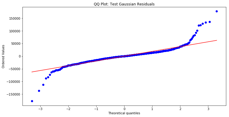
Here we see that we have fat tails, and the data is not Gaussian at the tails. We thus have to be careful if we implement a t-test to test whether elements of $\hat{\boldsymbol{\beta}}$ are non-zero, as our test statistic requires that $\hat{\beta}$ is Gaussian. Gaussian errors would imply a Gaussian $\hat{\beta}$ , but since we don’t have Gaussian residuals, we don’t have Gaussian errors, and we need to see whether the central limit theorem can tell us that $\hat{\beta}$ is approximately Gaussian. We must investigate this carefully before concluding so. There are three common ways to deal with normality violations other than invoking the central limit theorem: 1) transform either your features or your response 2) fit a GLM instead of doing linear regression 3) bootstrapping.

Heteroskedasticity

Next we check whether we have homoskedasticity (equal variance in our error terms) or heteroskedasticity (unequal variance). Heteroskedasticity is a problem because it implies that the OLS estimator is no longer BLUE (best linear unbiased estimator) and some other estimators may have lower variance.

A first step is to plot the predicted values $\hat{y}_i$ on the training dataset vs the residuals $\hat{y}_i-y$ . If we see that the magnitude of $\hat{y}_i-y$ varies with $\hat{y}_i$ , this may indicate heteroskedasticity.

plt.plot(y_hat,y_np-y_hat,'o')
plt.xlabel(r'Predicted ')
plt.ylabel(r'Residuals ')
plt.title('Predicted vs Residuals')
plt.tick_params(axis='x')
plt.tick_params(axis='y')

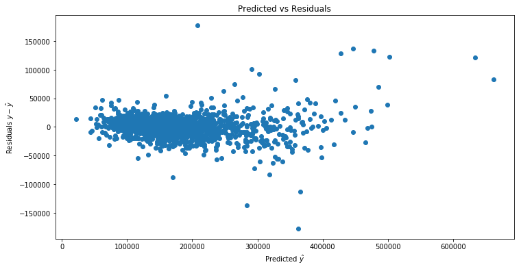
It looks like the magnitude is increasing as a function of the predicted. Next we fit a linear model regressing $(y_i-\hat{y})^2$ on $X^{(i)}$ . We then plot the predicted squared residuals $\hat{SR}_i$ vs $(y_i-\hat{y})^2$ to see if there is a relationship.

resid_model = OLS((y_np-y_hat)2,X_train_np) 
results_resid = resid_model.fit() 
resid_predict = resid_model.predict(results_resid.params) 
plt.plot(resid_predict,(y_np-y_hat)2,'o')

abline(1, 0)
plt.xlabel('Prediction of Squared Residual')
plt.ylabel('Squared Residual')

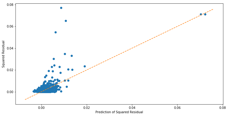
It looks like there is a relationship, and that $\boldsymbol{X}$ is predictive of $(y-\hat{y})^2$ . We can make this more formal by conducting a Breusch pagan test for whether regressing $(y-\hat{y})^2$ on $\boldsymbol{X}$ via OLS has significant coefficients. If it does, then we reject the null hypothesis of homoskedasticity in favor of heteroskedasticity.

from statsmodels.stats.diagnostic import het_breuschpagan
lm, lm_pvalue, fvalue, f_pvalue = het_breuschpagan(y_np-y_hat,X_train_np)
print 'the p-value for the lagrange multiplier test statistic is %f' % (lm_pvalue)


the p-value for the lagrange multiplier test statistic is 0.000000

Thus we reject the null hypothesis in favor of heteroskedasticity.

Independence

The last assumption is that the error terms are independent. If $\epsilon_i$ depends on $X^{(i)}$ or $y_i$ , then the errors are not independent (since observations with similar $X^{(i)}$ or $y_i$ will have similar $\epsilon_i$ ). Based on our investigation of heteroskedasticity, it is unlikely that the residuals are independent, and thus unlikely that the error terms are.

For data arriving in time, assuming Gaussian error terms, we can also test for autocorrelation.

The Five Linear Regression Assumptions: Testing on the Kaggle Housing Price Dataset

Linearity

Multicollinearity

Gaussian Residuals Test

Heteroskedasticity

Independence

Leave a Reply Cancel reply

Linearity

Multicollinearity

Gaussian Residuals Test

Heteroskedasticity

Independence

Related Posts

Leave a Reply Cancel reply