Fundamentals of Exponential Families

In this post we describe exponential families. We first motivate them via the problem of density estimation and wanting to match empirical moments to theoretical ones. We then describe why we might want to maximize entropy, and how exponential families maximize entropy for a given set of sufficient statistics. Next we describe how the choice of base measure and thus the support (subset of domain giving non-negative density values) allows exponential families to flexibly handle different types of data. We then show an example on a diabetes dataset, and conclude with a brief discussion of when to use an exponential family for density estimation and some of their limitations.

Motivation: Density Estimation with Moment Matching

A common problem in machine learning and statistics is density estimation: given iid samples $X_1,\cdots,X_n\in S$ , estimate a statistical model $p_\theta:S\rightarrow\mathbb{R}_{\geq 0}$ from a family of densities $\mathcal{P}=\{p_\theta:\theta\in \Theta\}$ . This lets us describe how likely different values of data are, including values we haven’t observed. It also lets us state the probability of an observation falling in some interval. For instance, what is the probability of a diabetes patient having glucose above or below some threshold? A natural question is: how do you choose the family $\mathcal{P}$ that we estimate a statistical model from?

Before we answer this, we might want to recall that one way data analysts, including statisticians and machine learning users and researchers, describe raw data, is in terms of summary statistics, particularly (empirical) moments. The raw theoretical moments are $\mathbb{E}X,\mathbb{E}X^2, ,\mathbb{E}X^3$ , etc. Their empirical counterparts are $\frac{1}{n}\sum_{i=1}^n X_i,\frac{1}{n}\sum_{i=1}^n X_i^2$ , etc. A natural attractive property then would be to do density estimation such that the theoretical moments of our estimated density match our empirical moments of the data we used to estimate it, so that $\mathbb{E}X=\frac{1}{n}\sum_{i=1}^n X_i , \mathbb{E}X^2 = \frac{1}{n}\sum_{i=1}^n X_i^2$ , etc. However there are still infinitely many such distributions with this constraint. We thus need further restrictions.

Maximizing Entropy while Moment Matching

One further desirable property would be for a density to make the weakest assumptions, given that the theoretical moments match the empirical ones. We need to quantify this, and can do so if we have a measure how much information content a density has about the value of a random variable. We then want to have the least information about the random variable’s value, given the moment matching constraint. A common measure of information content is Shannon entropy. Maximizing Shannon entropy subject to moment constraints does lead to a unique solution, and one can describe the family of such solutions as exponential family densities. The optimization problem is then

(1) $\begin{align*}\arg\max_p \Omega(p)&=\int_S p(x)\log p(x)dx\\&s.t.\\\mathbb{E}[\phi_k(X)]&=\frac{1}{n}\sum_{i=1}^n \phi_k(X_i),k=1,\cdots,K\end{align*}$

The first line tells us that we want to find the density to maximize the entropy, or uncertainty about the value of the random variable. The second line is the constraint that the expected summary statistics match their empirical counterparts. In the most common (univariate) exponential families we choose these to either be $\phi(x)=(x)$ (e.g. Poisson, exponential, Bernoulli, negative binomial) or $\phi(x)=(x,x^2)$ (e.g. Gaussian). Other cases include $\phi(x)=(\log x)$ (Pareto) and $\phi(x)=(x^k)$ (Weibull). In principle one could also specify a rich set such as monomials $\{x^k\}_{k=1}^K$ or Fourier basis functions to obtain very flexible densities, but this leads to some mathematical difficulties in practice and is rarely done.

The solution to this optimization problem has the form

(2) $\begin{align*}p(x)&=\exp(\theta^T \phi(x)-A(\theta))\end{align*}$

for some parameters $\theta\in \mathbb{R}^K$ where $A(\theta)$ ensures that the density integrates to $1$ . In practice (there is a theoretical reason for this but it’s a bit inelegant to handle as the solution to the optimization problem without using measure theory) we often see exponential families written as

(3) $\begin{align*}p(x)&=h(x) \exp(\theta^T \phi(x)-A(\theta)) \end{align*}$

where $h(x)$ is known as the base measure. Thus an exponential family has several parts:

$h:S\rightarrow \mathbb{R}$ : base measure
$\theta\in \mathbb{R}^k$ : parameters
$\phi:S\rightarrow \mathbb{R}$ : sufficient statistics
$A(\theta)$ : log-normalizer

Handling Different Types of Data with the Base Measure

While having a max entropy density subject to moment constraints is a desirable property, we’d like one (or more by choice of constraints) each for different data types: real-valued (Gaussian), count-valued (Poisson), positive real-valued (exponential), etc. This is where $h(x)$ the base measure comes in.

An important concept here is the support of a density $p$ : the subset of the domain such that $p(x)>0$ . For real-valued data we want this to be the real line $\mathbb{R}$ . For count-valued data we want it to be the counting numbers $\mathbb{N}$ . Since the exponential function is always positive, $p(x)$ inherits its support from $h(x)$ . Thus we choose $h(x)$ to have the support appropriate for the type of data we’re handling. As an example, for a Bernoulli density where we want the support to be $\{0,1\}$ , we would let $h(x)=I(x=0)+I(x=1)$ . This gives us that $p(x)=0$ if $x\not\in \{0,1\}$ .

Example: Diabetes Biomarker

Here we look at the response value of a dataset from a classic paper [1]. This is ‘a quantitative measure of disease progression one year after baseline.’ Unfortunately not much more information is given. We will investigate it and fit an exponential family density. We start by importing libraries and the relevant dataset:

from sklearn.datasets import load_diabetes
from matplotlib import pyplot as plt
import numpy as np
from scipy.stats import gamma

data = load_diabetes()['target']
data = data

We then create a histogram of the data of interest.

plt.hist(data)

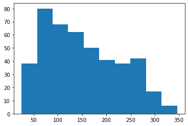
We can check what kind of observation values (natural numbers) the data takes to decide what kind of density to fit.

np.unique(data)

array([ 25.,  31.,  37.,  39.,  40.,  42.,  43.,  44.,  45.,  47.,  48.,
        49.,  50.,  51.,  52.,  53.,  54.,  55.,  57.,  58.,  59.,  60.,
        61.,  63.,  64.,  65.,  66.,  67.,  68.,  69.,  70.,  71.,  72.,
        73.,  74.,  75.,  77.,  78.,  79.,  80.,  81.,  83.,  84.,  85.,
        86.,  87.,  88.,  89.,  90.,  91.,  92.,  93.,  94.,  95.,  96.,
        97.,  98.,  99., 100., 101., 102., 103., 104., 107., 108., 109.,
       110., 111., 113., 114., 115., 116., 118., 120., 121., 122., 123.,
       124., 125., 126., 127., 128., 129., 131., 132., 134., 135., 136.,
       137., 138., 139., 140., 141., 142., 143., 144., 145., 146., 147.,
       148., 150., 151., 152., 153., 154., 155., 156., 158., 160., 161.,
       162., 163., 164., 166., 167., 168., 170., 171., 172., 173., 174.,
       175., 177., 178., 179., 180., 181., 182., 183., 184., 185., 186.,
       187., 189., 190., 191., 192., 195., 196., 197., 198., 199., 200.,
       201., 202., 206., 208., 209., 210., 212., 214., 215., 216., 217.,
       219., 220., 221., 222., 225., 229., 230., 232., 233., 235., 236.,
       237., 241., 242., 243., 244., 245., 246., 248., 249., 252., 253.,
       257., 258., 259., 261., 262., 263., 264., 265., 268., 270., 272.,
       273., 274., 275., 276., 277., 279., 280., 281., 283., 288., 292.,
       293., 295., 296., 297., 302., 303., 306., 308., 310., 311., 317.,
       321., 332., 336., 341., 346.])

We can see that the data takes natural number values. However given that the original paper used linear regression and from its brief description, we presume that these are actually real-valued but we have natural numbers due to coarse measurement. Since the data exhibits skewness, we can try fitting a gamma density and plotting the fitted density along with a histogram density estimate.

fit_alpha, fit_loc, fit_scale = gamma.fit(data)
k = np.arange(np.min(load_diabetes()['target']),np.max(load_diabetes()['target']))

plt.plot(np.arange(-10,np.max(data)+10),gamma.pdf(np.arange(-10,np.max(data)+10), fit_alpha,fit_loc,fit_scale),label='Gamma Fit')
plt.hist(data,density=True,color='b',alpha=0.1,label='Histogram')
plt.xlim(np.min(data),np.max(data))
plt.title('Exponential Family Fit vs Histogram')
plt.legend()

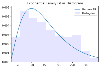
For a parametric distribution this is a fairly good fit. It captures the mode relatively well as long as the skewness and decay.

Discussion

In this post we gave a brief introduction to exponential family densities. We motivated them as densities doing moment matching while trying to keep assumptions to a minimum (maximize entropy), and described how the choice of base measure affects the support and thus what kind of data the density can handle. We then showed an example of density estimation with a diabetes biomarker. A major limitation of the exponential family framework is in handling densities with many modes. This can be done via a sufficiently rich choice of $\phi(x)$ , but leads to difficulties in computing $A(\theta)$ . [2] provides a discussion. However, it is often simpler (at least in low dimensions) in those cases to either use mixture models or kernel density estimation.

[1] Efron, Bradley, Trevor Hastie, Iain Johnstone, and Robert Tibshirani. “Least angle regression.” The Annals of statistics 32, no. 2 (2004): 407-499.
[2] Cobb, Loren, Peter Koppstein, and Neng Hsin Chen. “Estimation and moment recursion relations for multimodal distributions of the exponential family.” Journal of the American Statistical Association 78, no. 381 (1983): 124-130.

Motivation: Density Estimation with Moment Matching

Maximizing Entropy while Moment Matching

Handling Different Types of Data with the Base Measure

Example: Diabetes Biomarker

Discussion

Related Posts

Leave a Reply Cancel reply