Decision Trees, Entropy, and Information Gain

Contents hide

1 Why Use a Decision Tree?

2 Learning Decision Trees

3 Information Theory Background

3.1 Information Content

3.2 Entropy

3.3 Information Gain

3.4 Tying Back to Decision Trees

4 An Example: The Iris Dataset

5 Discussion

An important class of machine learning models is decision trees: you can use them for both classification and regression. In this post we first define decision trees. We then describe their advantages, followed by a high-level description of how they are learned: most specific algorithms are special cases. Next we describe several ideas from information theory: information content, entropy, and information gain. Finally we show an example of decision tree learning with the Iris dataset.

Decision trees involve a hierarchy of if/else statements. Each if/else node of the tree either terminates with a value or triggers another if/else statement. Generally the if/else statement involves thresholding features.

Decision trees can summarize the way humans reasons. For example, in deciding whether the probability of Covid is high enough to warrant testing, if/else statements could look like:

Does this patient have a temperature above some threshold?
Do they have a cough?
Does this patient have difficulty breathing?
Is the number of Covid cases relative to the population in this region above some threshold ?

When such questions are arrange in a hierarchical structure this becomes a decision tree.

Why Use a Decision Tree?

The most obvious reason to use a decision tree is its ease of interpretation. For any decision (which in this case is a classification or regression output), one can trace the steps that led to that decision, and look at how changing a single variable would have changed the decision made. This tracing can be done using the visualization of the tree, which is very intuitive.

The main competing interpretable models are linear regression and generalized linear models (GLMs). A major advantage of decision trees is how interaction terms are handled. In GLMs, of which linear regression is a special case, one has to specify which interaction terms to include by hand. With enough features, it becomes difficult to decide which interaction terms to include in order to trade off model richness vs potentially overfitting. Decision trees learn which interactions are important automatically by simply sequentially looking at features in order to arrive at a decision.

Decision trees also involve fewer statistical assumptions to think carefully about. For instance, a nice property of ordinary least squares (OLS) is that it gives the best linear unbiased estimator (BLUE), which in some cases implies a good fit and helps it make good predictions. However, that only holds if the relationship between features and response is linear and the errors are uncorrelated and homoskedastic (have equal variance). Decision trees make fewer assumptions, although they also are less studied theoretically.

Finally, decision trees have some robustness to class imbalance. When the minority class always has features in the same region of feature space, decision trees are effective at identifying this. However, when the features are in different regions, this does not necessarily work.

Learning Decision Trees

Most decision tree learning algorithms are some variant of the following high-level algorithm. The key idea is that at each step, one cycles through features and then does the following:

Check which feature improves some metric the most (information gain, gini impurity)
Check which threshold for the split improves the metric the most
Split on that feature+threshold pair
Continue until some termination condition is met
1. max depth, no more features, everything belongs to same class, no examples satisfying

Before moving forward, let’s import some libraries that we will use in our experiments

from sklearn import datasets, tree
import numpy as np
from matplotlib import pyplot as plt
from scipy import stats

Information Theory Background

In this section we will give a crash course on some information theory relevant to decision trees. The key idea is that one metric to split on is information gain or mutual information.

Information Content

The information content in an observation describes how surprising it is, given the distribution it comes from. More formally, let $x\in \mathcal{X}$ be an observation coming from a random variable with probability mass function $p:\mathcal{X}\rightarrow [0,1]$ . Then the information content of $x$ is $I(x)=-\log p(x)$ . Thus high probability outcomes are associated with low values and low probability outcomes with high values.

One might ask why take a $\log$ ? Why not simply take $-p(x)$ . The reason is that the latter maps to $[-1,0]$ while $-\log p(x)$ maps to $[0,\infty]$ . Having the smallest possible information content be $0$ and the max be $\infty$ is very intuitive. Having the smallest information content be $-1$ and the max be $0$ is less so.

Let’s look at this visually. We can take two $\textrm{binom}(50,p)$ random variables: one has $p=0.5$ and the other $0.8$ . We then plot their information content for values $0$ to $50$ .

x=np.arange(50)
plt.plot(x,-np.log(stats.binom.pmf(x,50,0.5)),label='Binom(50,0.5)')
plt.title('Information Content')
plt.xlabel('Value')
plt.ylabel('Information Content')
plt.plot(x,-np.log(stats.binom.pmf(x,50,0.8)),label='Binom(50,0.8)')
plt.legend()

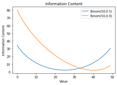
Information content for two Binomial random variables at different observation values.

Noting that the mode with $p=0.5$ is 25 and the mode with $p=0.8$ is 40, we see that the mode, the value with the highest probability, has the lowest information content: it is least surprising when it occurs. This make sense intuitively. We also see that values with lower probability have higher information content: they are more surprising.

Entropy

The entropy of a random variable is the expected information content. This can be framed intuitively in several ways:

What is the expected surprise of the outcome of this random variable?
How much uncertainty is there in the random variable?
How much information would we gain if we knew the value of the random variable?

Mathematically, the entropy is

(1) $\begin{align*}H(x)&=\mathbb{E}[I(X)]=\mathbb{E}[-\log p(x)]\end{align*}$

For a Bernoulli random variable, we can plot the entropy as a function of $p$ .

plt.plot(np.arange(101)*.01,stats.binom.entropy(1,np.arange(101)*.01))
plt.title('Entropy as a Function of p for Bernoulli')
plt.xlabel('p')
plt.ylabel('Entropy')

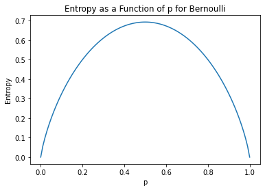
Entropy for a Bernoulli random variable as a function of the success probability.

We see that at $p=0$ and $p=1$ we have the lowest entropy. This make sense intuitively: there is no uncertainty at those point. As $p$ moves closer to $0.5$ the uncertainty increases and attains a maximum at $p=0.5$ .

A related important concept is the conditional entropy. Intuitively, this is the expected surprise of the outcome of a random variable $X$ , given that we know the outcome of some other random variable $Y$ . Mathematically it is

(2) $\begin{align*}H(X|Y)&=\mathbb{E}_{p(X,Y)}[-\log p(X|Y)]\end{align*}$

Information Gain

One metric used to split on is information gain which is also called mutual information. Intuitively this tells how much knowing the value of a random variable $Y$ reduce the uncertainty about another random variable $X$ . Mathematically this is

(3) $\begin{align*}I(X,Y)&=\sum_{y\in \mathcal{Y}}\sum_{x\in \mathcal{X}}p_{X,Y}(x,y)\log\frac{p_{X,Y}(x,y)}{p_X(x)p_Y(y)}\end{align*}$

From this we can show

(4) $\begin{align*}I(X;Y)&=H(X)-H(X|Y)\end{align*}$

which says that the mutual information of $X$ and $Y$ is the entropy of $X$ minus the conditional entropy of $X$ given $Y$ . More intuitively, this is saying that the mutual information is the difference in expected surprise of $X$ when we don’t know $Y$ vs when we do.

Tying Back to Decision Trees

We can tie this back to learning in decision trees: at each stage of the process, we split on the variable that maximizes mutual information with the target value. That is, the variable that reduces are uncertainty about the target by the most. Say $Y$ is the target value and we have $X_1,\cdots,X_p$ . Then we check $I(Y;X_1),\cdots,I(Y;X_p)$ . We generally can’t compute these in closed form without knowing the distributions, but we can approximate them using sampling and in some cases other methods: sklearn’s mutual_info_classif is one implementation. Once we know the $X_i$ that we want to split on, we need to choose a threshold. We again choose the threshold that maximizes mutual information by minimizing conditional entropy.

An Example: The Iris Dataset

We now show an example on the iris dataset. This is a dataset of flowers where the attributes are sepal and petal length and width in centimeters. This has three classes with 50 observations for each class. We first load the dataset.

data = datasets.load_iris()
X=data['data']
y=data['target']

Now we can fit a tree and plot it

#create tree
clf = tree.DecisionTreeClassifier('entropy')
#fit it to the iris dataset
clf.fit(X,y)

#plot the tree
fig, ax = plt.subplots(figsize=(100, 100))
tree.plot_tree(clf,ax=ax,feature_names=['sepal length','sepal width','petal length','petal width'])
plt.show()

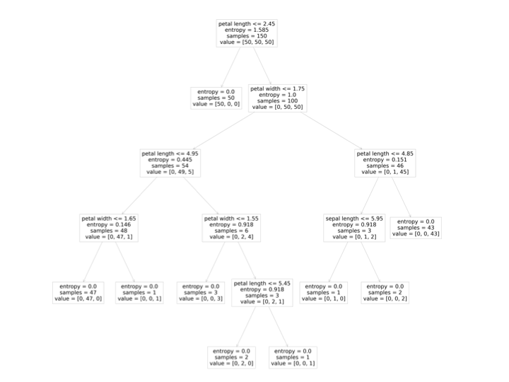
Then for any classification decision we make we can trace how we got there. For example, say we have a new observation with petal length 3, width 1, sepal length 6, and sepal width 2. Then we will move right, left, left, left. This will put us in the second class, Versicolour.

Discussion

In this post we described decision trees. We described why to use them, the high-level idea for all algorithms to learn them, some information theory background, and then showed an example.