In this post we describe the fundamentals of using ARIMA models for forecasting. We first describe the high level idea of ARIMA models. We then describe autoregressive models, integration, and moving average models separately briefly. Following this, we show how to fit an ARIMA models to data.
Fundamentals
ARIMA standards for autoregressive integrated moving average. The autoregressive part of the model describes the effect of persistent shocks. The MA terms describe the effect of shocks with short term effects. Finally, the integration involves differencing a series to remove or reduce trend and seasonal effects.
Autoregressive Model
Autoregressive models describe the effect of persistent shocks by regressing current values of a time series on lagged values. For instance, exercise may have a persistent (albeit decaying) effect on blood sugar levels. Given a time series  , an AR(p) model is
(1) 
we can alternatively write this using the backshift operator 
(2) 
where  and
and  .
.
Moving Average Model
A moving average model describes the effect of short term shocks by expressing the current value of a time series as a sum of the current plus a linear combination of past white noise terms. For instance, drinking a sugary drink would normally have a short term effect on blood sugar levels that does not persist over the long run (unless one drinks huge amounts). We can express this as
(3) 
which we can equivalently write as
(4) 
Note that a moving average model is different from moving average smoothing. The first is used to describe the effect of short term shocks, while the second is used to remove the effects of noise and isolate trend and seasonality.
Autoregressive vs Moving Average Models
The autoregressive vs moving average models describe the effects of different types of shocks: long run vs short run, respectively. From a statistical perspective, this expresses itself in the autocorrelation function. For a stationary AR(p) process, the autocorrelation function  for all
  . For an AR(1) process, this takes the form
  . Since we need
  for a causal process, this is geometric (fast) decay, but nevertheless the effect of an autoregressive shock lasts forever. In contrast, for an MA(q) process,
  only if
  .
.
Integration
ARMA models are only appropriate for weakly stationary series (i.e. first and second moments are constant). For a covariance stationary series, one can demean the series by repeatedly differencing it. One can think of it in terms of a mean function: for many classes of functions, high enough order derivatives will be  . We can take the same idea for discrete time series by differencing
  times.
Applying it in Practice
We’ll first load two libraries and then look at the varve time series of glacial varve thickness.
library(astsa)
library(forecast)
Our first goal is to deal with a weakly stationary time series where effects of previous lags and errors are linear. Let’s first look at the lag plot to see whether there is non-linearity or non-constant variance
lag1.plot(varve,9)
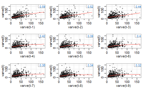
We see funnel behavior, which suggests non-constant variance, and non-linearity where it looks like the slope is decreasing. We can apply a log transform to see if that helps.
lag1.plot(log(varve),9)
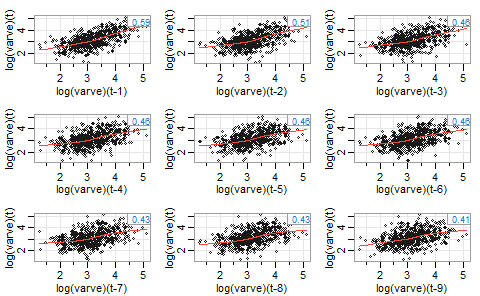
This greatly decreases the funnel behavior and seems to reduce the non-linearity as well. Now let’s check the ACF plot of the logs. We want rapid decay and no obvious seasonality.
acf(log(varve))
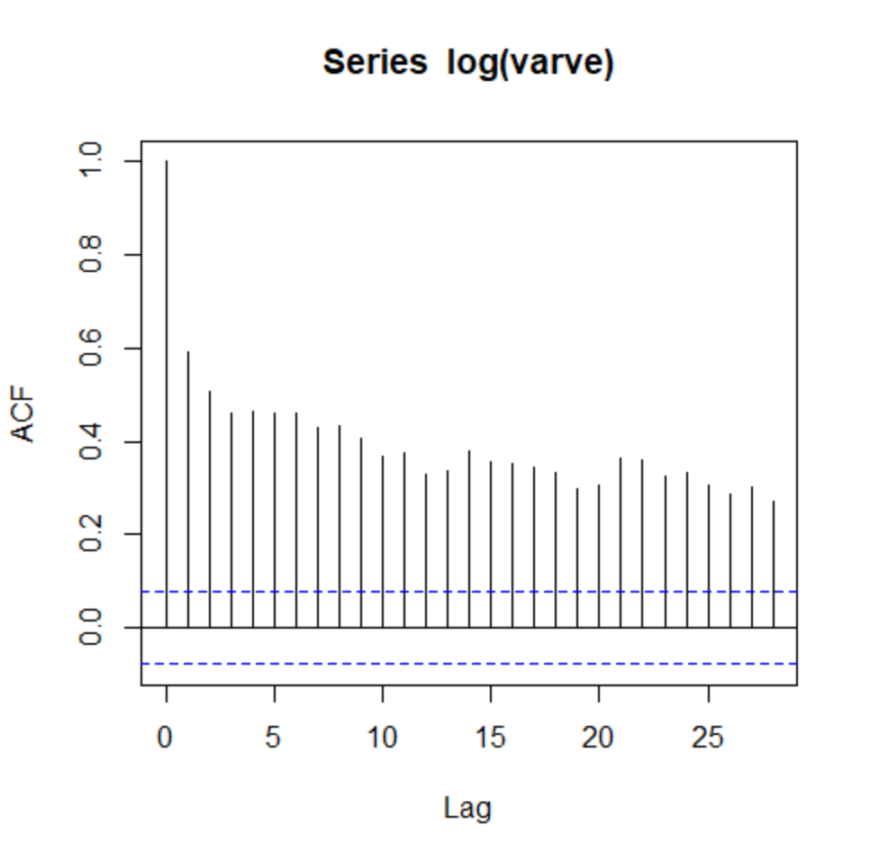
This decay is very slow, suggesting that the mean function is not constant. Let’s try first differencing to see if that improves it.
acf(diff(log(varve)))
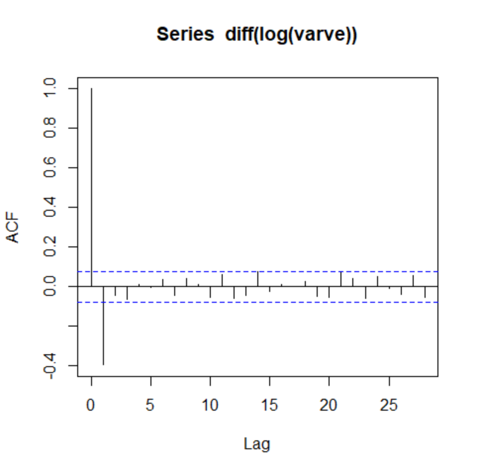
This helps a lot. Thus we select d=1 for a model that is integrated of order 1. We still need to select p for the number of AR terms and q for the number of MA terms. The previous plot shows one significant lag in the ACF plot, suggesting q=1. We can then use a PACF plot to decide the number of AR terms.
pacf(diff(log(varve)))
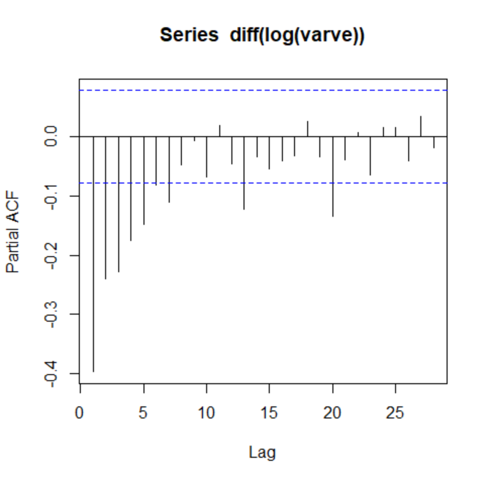
We see that the first five lags are significant. We thus have p=5,d=1,q=1. Let’s try fitting it and checking the residuals
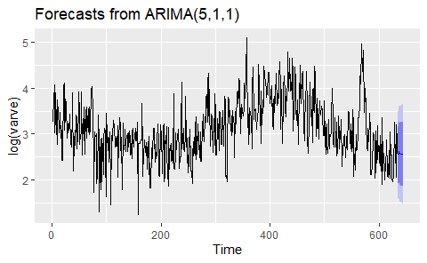
fit <- Arima(log(varve), order=c(5,1,1))
checkresiduals(fit)
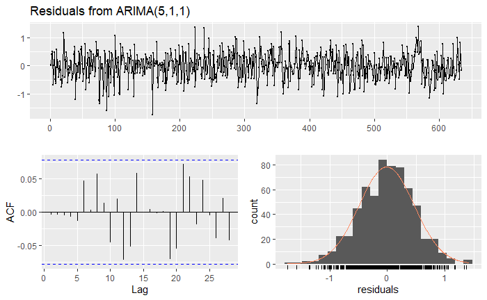
Their behavior looks like white noise, as desired. We can now look at forecasts.
autoplot(forecast(fit))