Attention Mechanisms: A Geometric View

Introduction

In this post we describe attention mechanisms by motivating it using geometric intuition. The ideas are largely based on two somewhat theoretical papers: [1] and [2], but we focus on the core intuition from those papers rather than the theory.

A classic technique in both machine learning and statistics is to take weighted averages as a pre-processing step. For instance, in time series, one might take a moving average of the time series to smooth it. Based on the importance of neighboring information, this could assign uniform weights (simple moving average) or have different types of decay of importance as a function of time. In image data, convolutions perform a similar task. However, they are strictly speaking a not expectations since the weights may not make a valid probability mass function (pmf). These convolutions can blur an image or magnify important aspects of the image.

One extension of these ideas is to let the weights themselves be a mapping from the input objects that one takes a weighted average over to a vector of weights. In time series, this would mean that the moving average weights for a sliding window are themselves a mapping from the sliding window. They then vary as we move the sliding window. We’d like to choose these weights to achieve two tasks. The first isto reflect the ‘importance’ of specific locations (times, pixel locations). The second is to help achieve good performance in prediction tasks. This is the core basic motivation of the attention mechanisms in use today.

Outline

We start by defining an attention mechanism, describing why choosing the attention weights is the key challenge. Next we describe a very naive idea: choosing the attention weights to point in approximately the same direction as the input vector (sliding window). We describe a first attempt at this, maximizing the between the attention weights and the input vector, and why this doesn’t actually lead to pointing in approximately the same direction, and that it will also fail for multi-dimensional observations.

Following this naive idea, we then argue that adding a regularizer (for instance Shannon entropy) to the optimization problem does lead to pointing in approximately the same direction. This idea is too naive in practice and will also fail for multi-dimensional observations, but by replacing the data with another representation or summary, we obtain a workable idea that is in fact what many attention models use. With these two extensions to a very naive idea, we can recover softmax attention in the form that many papers use today. Again, these ideas primarily come from [1] and [2] but are presented in a much more mathematical way.

What is an Attention Mechanism

An attention mechanism involves three parts, and refers to calculation of the first. 1) a context vector 2) an attention weight probability mass function (pmf) 3) a value function. The context vector is given by

(1) $\begin{align*}c&=\mathbb{E}_p[V(T)]\end{align*}$

The parts are as follows:

The context vector $c$ is a weighted average of a representation $V(t)$ of data. This is used as input to a prediction model, such as a neural network.
$t\in S$ is a location in the domain or set of locations $S$ . $S$ could be the set of times in a sliding window, a set of pixel locations, etc.
The attention weights $p\in \mathbb{R}^{|S|}$ , which is a discrete pmf describing the importance of locations $t\in S$ .
$T\in S$ is a random variable drawn from $p$ .
$V:S\rightarrow\mathbb{R}^d$ is a representation of the data at location $t$ .

Intuitively, $V(t)$ might be a vector representation of a word at position $t$ in a sequence, and we’re interested in taking a weighted average over a sequence of words and use that to perform some prediction task such as predicting the next word, classifying a sentence or document, etc.

The important question is what should p the attention weights be? What properties do we want $p$ to have, and how do we formulate $p$ as the solution to an optimization problem so that it has these properties? Intuitively, we would like weights that help us make good predictions.

Naive Attention Weights

One very naive idea, which it turns out is surprisingly close intuitively to what attention models do in practice, is make ‘ $p$ similar to $x$ ,’ our data that we are taking a weighted average over. A good start would be using unnormalized cosine similarity or $l^2$ inner product and trying to maximize that, subject to the constraint that $p\in \Delta^{|S|}$ the simplex i.e. $p$ is non-negative and sums to $1$ . This ‘hopefully’ makes $p$ point in approximately the direction of $x$ .

The optimization problem for this is

(2) $\begin{align*}\arg\max_{p\in \Delta^{|S|}}\langle p,x\rangle&=\arg\max_{p\in \Delta^{|S|}}\Vert p\Vert\Vert x\Vert\cos\gamma\end{align*}$

where $\gamma$ is the angle between $p$ and $x$ . This idea gives us a good direction to start with, but has some serious flaws:

It is too naive and would be unlikely to actually help prediction
We need $p$ and $x$ to lie in the same vector space. This only holds if $x$ is a set of scalars. If $x$ is a set of vectors (say vector representations of words, then this won’t hold).
It doesn’t actually make the optimal $p$ point in the direction of the data $x$ . By the fundamental theorem of linear programming, some standard basis vector $e_t$ will be a solution to the optimization problem. We can see this in the figure below.

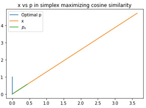As a first idea for attention weights $p$ , we wanted $p$ to point in approximately the direction of the data $x$ , but due to the fundamental theorem of linear programming, maximizing unnormalized cosine similarity doesn’t actually achieve this, as we see. It simply gives us $(1,0)$ . This is not very useful: is there some similar optimization problem that will give us a solution that *does* approximately point in the direction of the data?

Regularizing the Optimization Problem

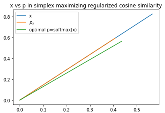
We can avoid the pitfall of having standard basis vectors as a solution by including a regularizer.

(3) $\begin{align*}\arg\max_{p\in \Delta^{|S|}}\langle p,x\rangle-\Omega(p)&=\arg\max_{p\in \Delta^{|S|}}\Vert p\Vert\Vert x\Vert\cos\gamma-\Omega(p)\end{align*}$

If we let $-\Omega(p)$ be Shannon entropy, then the solution to this is

(4) $\begin{align*}\arg\max_{p\in \Delta^{|S|}}\langle p,x\rangle-\Omega(p)&=\textrm{softmax}(x)\end{align*}$

which is very close to the softmax attention that many people use in practice. However, they tend not to use the original data $x$ , but instead use some transformation or summary of it. Let’s look at what the solution looks like again in the 2d case.

By including a regularizer (negative Shannon entropy) in the optimization problem, we now have a unique solution that is *not* a standard basis vector. Further, the solution now points in approximately the direction of the data. Unfortunately, this is likely too naive to work in practice, and if $x$ and $p$ are not in the same vector space we cannot do this.

However, we still have the problem that if $x$ is a set of $|S|$ vectors instead of $|S|$ scalars, the inner product we used isn’t valid as it needs to be between two vectors.

Summarizing the Data

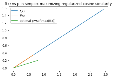
We can extend the naive attention weights by replacing $x$ with a vector summarizing or representing it. Instead of maximizing the regularized unnormalized cosine similarity between $p$ and $x$ , where the latter may be a matrix instead of a vector (which isn’t valid), we maximize the similarity between $p$ and a summary $f(x)$ of $x$ . The summary maps $f:\mathbb{R}^{|S|\times D}\rightarrow \mathbb{R}^{|S|}$ . This maps an $|S|\times D$ matrix to a vector of $|S|$ scalars. We then want to solve

(5) $\begin{align*}\arg\max_{p\in \Delta^{|S|}}\langle f(x),p\rangle_{l^2}&=\arg\max_{p\in \Delta^{|S|}}\Vert f_x\Vert\Vert p\Vert \cos\gamma\end{align*}$

We’re making a location ‘important’ i.e. giving it a large attention weight if its summary value is large in that direction, while constraining the attention weights to form a valid pmf. The next figure visualizes this.

By replacing $x$ (potentially a matrix) with another representation $f(x)$ (a vector), where $f$ will be learned, and making $p$ point in approximately that direction, we can now handle the case where $x$ is a matrix. We also gain flexibility that will be useful for our final prediction task, since $f$ will be learned end-to-end with the prediction model to help make good predictions.

Parametrizing the Summary

We still need a form for $f(x)$ . One simple form lets $f_t(x)$ be a linear combination of basis functions of $t$ . One can let the weights map from $x$ to a vector. This gives

(6) $\begin{align*}f_t(x)&=\theta^T(x)\phi(t),\theta:\mathbb{R}^{|S|\times D}\rightarrow \mathbb{R}^{M},\phi:S\rightarrow \mathbb{R}^{M}\end{align*}$

We can use a rich or a simple form for $\theta(x)$ , including a neural network, a linear transformation, or some other transformation, while maintaining a relatively simple linear form for $f_t(x)$ where we can easily do backpropagation.

The mapping $\phi(t)$ tell us about the ‘starting’ importance of different positions, before observing the data $x$ . For instance, in [3] they used $\phi(t)=e_t$ the canonical basis vectors. Intuitively, this says that before observing $x$ , you assign uniform importance to different locations. Then, the data updates this with $\theta(x)$ . We could also start with something else i.e. exponential decay, a kernel smoother, etc.

Softmax Attention

In practice most papers use some form of softmax attention. It turns out that this framing of maximizing the similarity (inner product) between the attention weights and a summary of the data, while penalizing the attention weights to be more uniform gives us softmax attention

(7) $\begin{align*}\textrm{softmax}(f)=\frac{\exp(f)}{\sum_{k=1}^{|S|}\exp(f_k)}\end{align*}$

Using an Attention Mechanism in a Prediction Model

The real power of an attention model comes from training it end-to-end along with a prediction model. We can learn both the model where we input $c$ and output predictions, and the parameters $\theta$ jointly. We’re thus learning a summary of the data such that when we use attention weights that are approximately in the direction of this summary to compute a weighted expectation of a data representation, we make good predictions.

[1] Martins, André, et al. “Sparse and Continuous Attention Mechanisms.” Advances in Neural Information Processing Systems 33 (2020).
[2] Blondel, Mathieu, André FT Martins, and Vlad Niculae. “Learning with Fenchel-Young losses.” Journal of Machine Learning Research 21.35 (2020): 1-69.
[3] Bahdanau, Dzmitry, Kyunghyun Cho, and Yoshua Bengio. “Neural machine translation by jointly learning to align and translate.” arXiv preprint arXiv:1409.0473 (2014).