Gradient Descent for Convex Optimization: The Basic Idea

Contents hide

3.1 Why are Convex Functions Important for Gradient Descent?

In this post we describe the high-level idea behind gradient descent for convex optimization. Much of the intuition comes from Nisheeth Vishnoi’s short course, but he provides a more theoretical treatment, while we aim to focus more on the intuition. We first describe why to use gradient descent. We next define convex sets and functions and then describe the intuitive idea behind gradient descent. We follow this with a toy example and some discussion.

Why Use Gradient Descent?

In many data analysis problems we want to minimize some functions: for instance the negative log-likelihood. However, the function either lacks a closed form solution or becomes very expensive to compute for large datasets. For instance, logistic regression lacks a closed form solution, while the naive closed form solution to linear regression requires solving a linear system, which may have stability issues. For the former, gradient descent provides us a method for solving the problem, while for the latter, gradient descent allows us to avoid these stability issues.

Convex Sets and Convex Functions

Much of the practical application and most of the theory for gradient descent involves convex sets and functions. Intuitively, a convex set is one where for any two points in a set, every point between them is also in the set. For example, consider a line in 1d from points $a$ to $b$ , and $x$ and $y$ are points on the line. Then any $z$ between them is also on that line. Thus a line is a convex set.

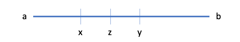
More formally, a convex set $\mathcal{K}$ is one where if $x,y\in \mathcal{K}$ , then for any $\lambda\in [0,1],\lambda x+(1-\lambda)y\in \mathcal{K}$ . In the previous case $\mathcal{K}=[a,b]$ and $z=x+(1-\lambda)y$ .

In the 1d case, a convex function is one where if you draw a line segment between the function evaluated at any two points, the line lies at or above the function everywhere in between. Let’s look at an example: the function $f(x)=x^4$ .

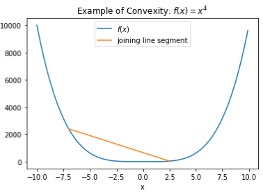
We see that the line segment joining the points $f(-7.5)$ and $f(2.5)$ lies above $f(x)$ for $x\in (-7.5,2.5)$ . We can also tell just from looking at it that this property would hold for the entire domain of the function. More formally, we have the following definition. For $x,y\in \mathcal{K}$ and $\lambda\in [0,1]$ , where $\mathcal{K}$ is a convex set, a function $f$ is convex if

(1) $\begin{align*}f(\lambda x+(1-\lambda)y)&\leq \lambda f(x)+(1-\lambda)f(y)\end{align*}$

here $\lambda f(x)+(1-\lambda)f(y)$ is the line segment between $f(x)$ and $f(y)$ , and $f(\lambda x+(1-\lambda)y)$ is the function, which lies below the line segment. In higher dimensions instead of the line segment lying above the function, the hyperplane lies above the function.

An equivalent definition of convexity for differentiable functions is that the tangent line or hyperplane to the function at any point lies below the function everywhere. The following plot of the same function illustrates this

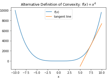
Again, we can see from looking at it that this property should hold for the function at any point. More formally, a differentiable function $f$ is convex if and only if for any $x,y\in \mathcal{K}$ , we have

(2) $\begin{align*}f(y)-f(x)&\geq \nabla f(x)^T(y-x)\end{align*}$

where $\nabla f(x)^T(y-x)$ is the inner product $\sum_{i=1}^d \nabla f(x)_i(y_i-x_i)$ .

Gradient Descent: Idea

The goal of gradient descent is to iteratively find the minimizer of $f(x)$ : $x^*=\arg\min_{x\in \mathcal{K}}f(x)$ for a convex function $f$ . The idea is to at each iteration use a linear approximation to $f(y)$ at a fixed $x$ , and minimize that. Consider the following approximation

(3) $\begin{align*}f(y)&\approx f(x)+\nabla f(x)^T(y-x)\end{align*}$

We want to minimize the right hand side in order to reduce $y$ . Since $x$ is fixed, we want to find $y$ to minimize $\nabla f(x)^T(y-x)$ . Generally we also start by assuming $\Vert y-x\Vert$ is fixed: that is we are only looking to move within a fixed distance. Since the distance between our next value $y$ and our current value $x$ is fixed, we only care about the direction we move.

We can note that the gradient is the direction in which the function grows fastest. Since we want to minimize, we want to move in the opposite direction of the gradient. Thus we can set

(4) $\begin{align*}y-x&=-\eta \nabla f(x)\end{align*}$

where $\eta>0$ is a constant. This moves in the opposite direction of the gradient, and it can be shown that for small enough $\Vert \eta\nabla f(x)\Vert$ this will move us closer to the minimizer $x^*$ .

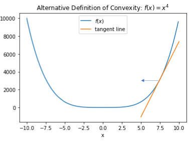
Let’s now look at example. Consider again the function $f(x)=x^4$ which we again plot below, and assume that we are currently at the point $x=7.5$ . Then the gradient at $x=7.5$ is positive. Thus if we move to the right, we are moving in the direction of the gradient, and if we move to the left, we move away from it and towards the minimizer. The intuition described above tells us to move left.

Now considering the fixed $x$ to be our current point $x_t$ , and the new $y$ to be our next point $x_{t+1}$ in an iterative algorithm, we obtain the following update, which can be used in several variants of gradient descent:

(5) $\begin{align*}x_{t+1}-x_t&=-\eta \nabla f(x_t)\\x_{t+1}&=x_t-\eta \nabla f(x_t)\end{align*}$

Why are Convex Functions Important for Gradient Descent?

For differentiable convex functions, the following three properties are equivalent:

$x$ is a local minimum of $f(x)$
$x$ is a global minimum of $f(x)$
$\nabla f(x)=0$

For gradient descent this is helpful because we can check when to terminate the algorithm by looking at the derivative and checking its magnitude. Further, we know that under this termination we have achieved (close to) the global minimum.

A Gradient Descent Example

Let’s try minimizing $f(x)=x^4$ using gradient descent. First we define functions to calculate both the function and its derivative.

import numpy as np
from matplotlib import pyplot as plt

def f(x):
    return x**4
def deriv_f(x):
    return 4*(x**3)

Then we will write code to run and plot the gradients over iterations.

x=7.5
gradient_magnitudes=[]
while(np.abs(deriv_f(x))>1e-4):
    grad = deriv_f(x)
    x=x-1e-3*grad
    gradient_magnitudes.append(grad)

plt.plot(gradient_magnitudes)
plt.xlabel('iteration')
plt.ylabel('gradient magnitude')
plt.title('Gradient Magnitude of Gradient Descent')

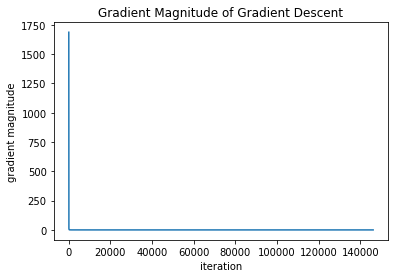
We can see fast convergence initially, but as the slope gets smaller, convergence gets very slow: the algorithm needs over 140,000 iterations with the learning rate we set. Further, if we increase the learning rate by a factor of 10, gradient descent diverges. In future posts we will investigate methods to deal with this.

Discussion

In this post we discussed the intuition behind gradient descent. We first defined convex sets and convex functions, then described the idea behind gradient descent: moving in the direction opposite the direction with the largest rate of increase. We then described why this is useful for convex functions, and finally showed a toy example.