In this post we describe how to analyze a scale location plot. You may also be interested in the fitted vs residuals plot, the residuals vs leverage plot, or the QQ plot.
The scale-location plot is very similar to residuals vs fitted, but simplifies analysis of the homoskedasticity assumption. It takes the square root of the absolute value of standardized residuals instead of plotting the residuals themselves. Recall that homoskedasticity means constant variance in linear regression. More formally, in linear regression you have
(1) 
where  is your design matrix,
  is your vector of responses, and
  your vector of errors. Homoskedasticity means that for each component
  of ,
of ,  .
.
The scale location plot has fitted values on the x-axis, and the square root of standardized residuals on the y-axis. Let’s look at a couple of plots and analyze them.
plot(lm(dist~speed,data=cars))
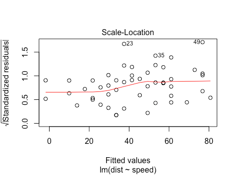
We want to check two things:
- That the red line is approximately horizontal. Then the average magnitude of the standardized residuals isn’t changing much as a function of the fitted values.
- That the spread around the red line doesn’t vary with the fitted values. Then the variability of magnitudes doesn’t vary much as a function of the fitted values.
We see that for this plot, the first condition is satisfied, while the second condition is a bit less clear. It’s likely still good enough to use though. We can do a Breusch Pagan Test to check for heteroskedasticity more formally.
library(lmtest)
model <- lm(mpg ~ disp + hp + wt + drat, data = mtcars)
bptest(model)

studentized Breusch-Pagan test

data:  model
BP = 3.2149, df = 1, p-value = 0.07297
Here the null hypothesis is homoskedasticity, and we fail to reject it.
Let’s look at another dataset
   library(mlbench)
   data(BostonHousing)
   plot(lm(medv ~ crim + rm + tax + lstat, data = BostonHousing))
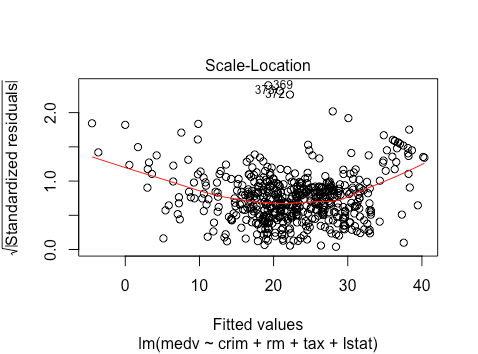
Here the scale location plot suggests some non-linearity here, but what we can also see is that the spread of magnitudes seems to be lowest in the fitted values close to 0, highest in the fitted values around 20, and medium around 40. This suggests heteroskedasticity. Let’s test it more formally again
model<-lm(medv ~ crim + rm + tax + lstat, data = BostonHousing)
bptest(model)

	studentized Breusch-Pagan test

data:  model
BP = 30.934, df = 4, p-value = 3.158e-06
We reject the null hypothesis of homoskedasticity with a p-value close to 0. As expected, there is strong heteroskedasticity.
You may also want to check out the fitted vs residuals plot, the residuals vs leverage plot, or the QQ plot.