In this post we describe how to interpret a QQ plot, including how the comparison between empirical and theoretical quantiles works and what to do if you have violations. You may also be interested in how to interpret the residuals vs leverage plot, the scale location plot, or the fitted vs residuals plot.
QQ-plots are ubiquitous in statistics. Most people use them in a single, simple way: fit a linear regression model, check if the points lie approximately on the line, and if they don’t, your residuals aren’t Gaussian and thus your errors aren’t either. This implies that for small sample sizes, you can’t assume your estimator  is Gaussian either, so the standard confidence intervals and significance tests are invalid. However, it’s worth trying to understand how the plot is created in order to characterize observed violations.
A QQ Plot Example
Let’s fit OLS on an R datasets and then analyze the resulting QQ plots.
model<-lm(dist~speed,data=cars)
plot(model)
The second plot will look as follows
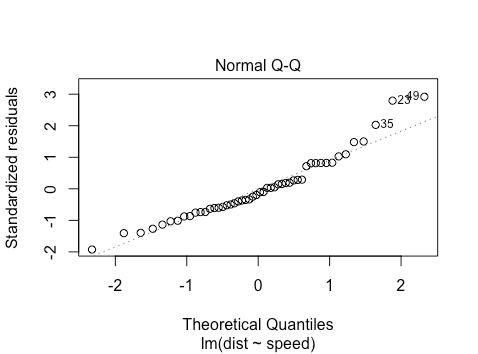
The points approximately fall on the line, but what does this mean? The simplest explanation is as follows: say you have some observations and you want to check if they come from a normal distribution. You can standardize them (mean center and scale variance to  ) and then ‘percentile match’ against a standard normal distribution. Then you can plot your points against a perfectly percentile-matched line.
In more detail, on the x-axis are the theoretical quantiles of a standard normal. That is, we sort the  points, and then for each
  , using the standard normal quantile function we find the
  so that
  . For this dataset, for the case of the leftmost point, we have that
  and
and  . Thus
qnorm(0.5/50)
 [1] -2.326348
which looks similar to where the leftmost point is on the x-axis. Intuitively, what this is saying is: we have 50 points and we want their x-values to be such that  . Based on the standard normal distribution, what x do we need to choose? For the y-axis, consider the empirical distribution function of the standardized residuals. We want our corresponding
  to be
to be  , but based on the empirical CDF of the standardized residuals.
Now how can we characterize the (slight) non-normality? What we see is that on the right hand side of the graph, the points lie slightly above the line. For the very right-most point, this is saying that the value such that  is larger under the empirical CDF for the standardized residuals than it is under a normal distribution. This suggests a ‘fat tail’ on the right hand side of the distribution.
Other Checks for Normality
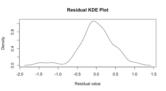
We can investigate further in three ways: a density plot, an empirical CDF plot, and a normality test. Note that one should generally do the former two after the qq plot, as it’s easiest to see that there are departures from normality in a qq plot, but it is sometimes easier to characterize them in density or empirical CDF plots. We can make a density plot as follows:
d<-density(model[['residuals']])
plot(d,main='Residual KDE Plot',xlab='Residual value')
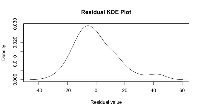
looking here, there appears to be some negative skewness along with a fat tail on the right. We can also make an empirical CDF plot.
plot(ecdf(model[['residuals']]))
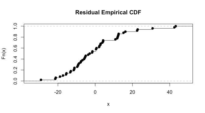
here it’s a bit difficult to say much. We can also do a normality test. I ‘suspect’ from looking at the plots that we’ll have a p-value in the .025-0.075 range, as there are clearly some violations but they don’t look extremely severe: let’s try the Shapiro test.
shapiro.test(model[['residuals']])

	Shapiro-Wilk normality test

data:  model[['residuals']]
W = 0.94509, p-value = 0.02152
The p-value is slightly outside the range I guessed but not by much. For a list of specific diagnostic cases to compare your plot to, see here.
What do you do If You Have Violations?
Transforming Data
Often one can transform data. For instance, if there is positive skewness, it may help to log transform the response. Let’s try this and analyze the qq plot, density, and the result of the Shapiro Wilks test again.
model<-lm(log(dist)~speed,data=cars)
plot(model)
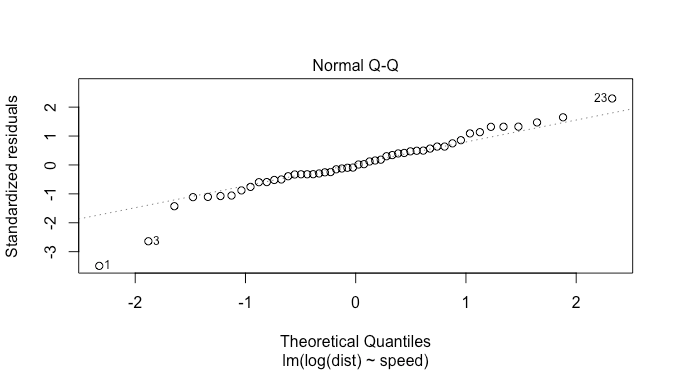
this looks a bit better, but there are now two points on the left suggesting fat tails: this is fewer than in the previous plot though. The density plot suggests this as well.
d<-density(model[['residuals']])
plot(d,main='Residual KDE Plot',xlab='Residual value')
Again, this may be slightly better than the previous case, but not by much.
shapiro.test(model[['residuals']])

	Shapiro-Wilk normality test

data:  model[["residuals"]]
W = 0.95734, p-value = 0.06879
This p-value is higher than before transforming our response, and at a significance level of  we fail to reject the null hypothesis of normality.
Other Methods
There are three other major ways to approach violations of normality.
- Have enough data and invoke the central limit theorem. This is the simplest. If you have sufficient data and you expect that the variance of your errors (you can use residuals as a proxy) is finite, then you invoke the central limit theorem and do nothing. Your
 will be approximately normally distributed, which is all you need to construct confidence intervals and do hypothesis tests.
 - Bootstrapping. This is a non-parametric technique involving resampling in order to obtain statistics about one’s data and construct confidence intervals.
- Use a generalized linear model. Generalized linear models (GLMs) generalize linear regression to the setting of non-Gaussian errors. Thus if you think that your responses still come from some exponential family distribution, you can look into GLMs.
Now that you’ve read about QQ plots, you may also be interested in how to interpret the residuals vs leverage plot, the scale location plot, or the fitted vs residuals plot.