In this post we analyze the residuals vs leverage plot. This can help detect outliers in a linear regression model. You may also be interested in qq plots, scale location plots, or the fitted and residuals plot.
To start with, what is leverage? Intuitively it describes how far a covariate  is from other covariates, and for linear regression it measures how sensitive a fitted
  is to a change in the true response
  . Let’s see the intuition for this with an example. Say we have the following
  and
and  values, describing a line through the origin with slope of
  .
.
   x=c(1,2,3,4,5,20)
   y=c(1,2,3,4,5,20)
   plot(x,y)
   abline(lm(y~x))
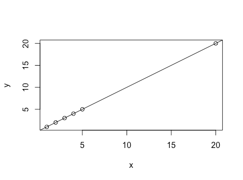
We notice that the  is further from the other points: it has high leverage. Thus changing the associated will change the model fit more than changing other points. Let’s try modifying the data by changing the
  to a
to a  , an increase in the value for that point of
  . That is, change the response for a covariate with low leverage. We plot the new line in green, while plotting the original line with the original points.
y=c(1,2,7,4,5,20)
abline(lm(y~x),col='green')
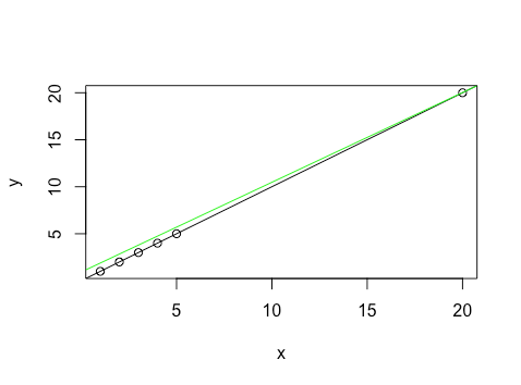
This barely gives us any change for the fitted at  . Now let’s try changing the value for the high leverage point by an increase of , while keeping all other points as in the original data. We plot the new line in red.
y=c(1,2,3,4,5,24)
abline(lm(y~x),col='red')

This leads to a much larger difference in the fitted for . We can see that high leverage or far covariates do in fact lead to a large change in fitted value in response to a change in the response.
Residuals vs Leverage
Now that we have some intuition for leverage, let’s look at an example of a plot of leverage vs residuals.
plot(lm(dist~speed,data=cars))
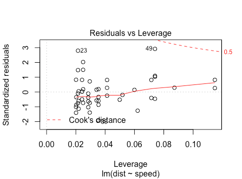
We’re looking at how the spread of standardized residuals changes as the leverage, or sensitivity of the fitted to a change in , increases. Firstly, this can also be used to detect heteroskedasticity and non-linearity. The spread of standardized residuals shouldn’t change as a function of leverage: here it appears to decrease, indicating heteroskedasticity.
Second, points with high leverage may be influential: that is, deleting them would change the model a lot. For this we can look at Cook’s distance, which measures the effect of deleting a point on the combined parameter vector. Cook’s distance is the dotted red line here, and points outside the dotted line have high influence. In this case there are no points outside the dotted line. For interpretation of other plots, you may be interested in qq plots, scale location plots, or the fitted and residuals plot.