Causality: Basics, Potential Outcomes, and Counterfactuals

Note: this is loosely based on Coursera’s A Crash Course on Causality: Inferring Causal Effects from Observational Data

Introduction

In many health problems, we want to describe the causal effect of a treatment or action $A$ on a response or outcome $Y$ . In the simplest setting $A$ takes values in $\{0,1\}$ , while $Y$ can be more flexible. We denote $A=1$ for the primary treatment and $A=0$ for either no treatment, a placebo, or an alternate treatment. For some examples:

$Y=1$ indicates a headache, $Y=0$ indicates no headache. $A=1$ indicates aspirin while $A=0$ indicates no treatment or a placebo.
$Y=1$ indicates death within some window due to myocardial infarction (heart attack). $Y=0$ indicates survival during that window. $A=1$ indicates surgery and $A=0$ indicates drug treatment.

We want to describe causality because we want to make decisions that lead to good outcomes. If $A$ is correlated with $Y$ but does not have a causal effect, making decisions for $A$ won’t help us achieve good health outcomes. For example, say we find that location predicts smoking behaviors. Under a causal relationship where location causes smoking, we expect that influencing where someone goes will influence their smoking behaviors. This gives us a powerful tool to help people reduce their smoking.

The gold standard for inferring causal effects is the randomized experiment. Here, subjects are randomized to different treatments. Under a ‘perfect’ design, it ‘forces’ inferred relationships to be causal. However, often randomized experiments are expensive, unethical, or impossible to conduct. In that case we would like to infer causal effects from observational data there is no experimental design to control $A$ . However, we’d like to say going forward what will happen to $Y$ if we control $A$ .

How to Get the Causality Wrong

If we aren’t careful and assign causation to variables that are simply associated with each other, we can get the causality wrong in a number of ways. Here are some common ones.

Spurious Correlation

In this setting, two variables are correlated, but do not have a causal relationship. This may be due to a confounder, or may simply be due entirely to chance.

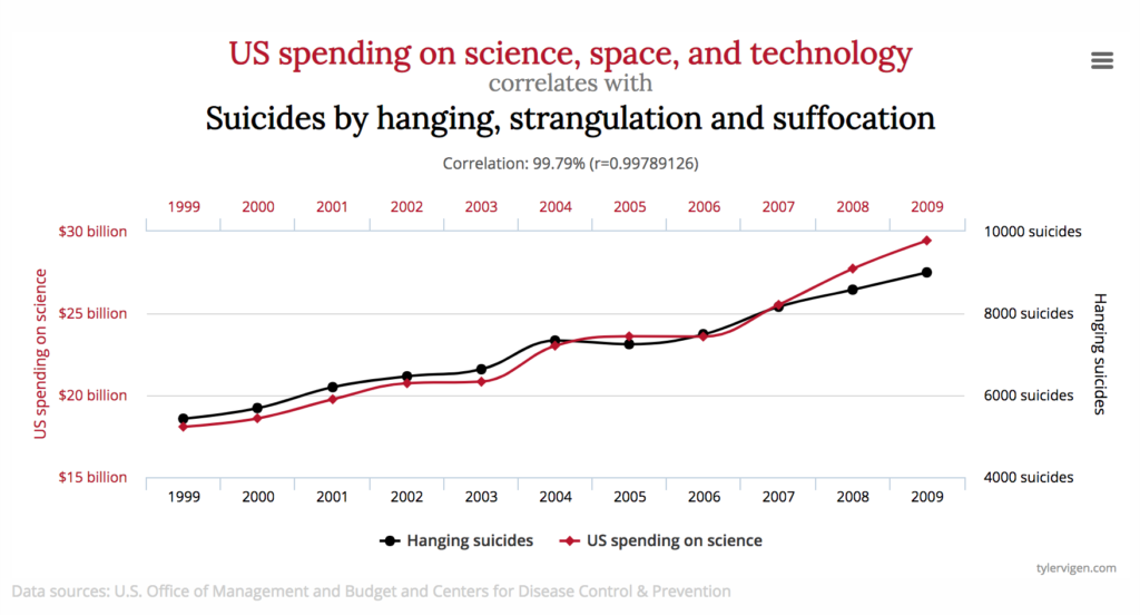
In the figure above we see that US spending on science space, and technology correlates with suicides by hanging, strangulation, and suffocation. It’s unlikely that one of these causes the other, or that they share a common causal factor (possibly population levels).

Reverse Causation

The direction of causation is wrong. An extreme example would be saying that heart attack surgery causes people to have heart attacks. Most reverse causation mistakes will tend to be more subtle.

A common example is in smoking: a smoker diagnosed with a serious disease such as cancer may quit smoking. This may lead to data saying that ex-smokers are more likely to die than current smokers: that is, quitting smoking causes high death risk. In reality high death risk caused them to quit smoking.

Confounder

Confounding variables can be of several types. We describe two of the most common. In one case, the confounding variable causes both variables in our model. For instance, if we have that murder and ice cream are correlated, it’s quite likely that neither causes the other. However, both of them are caused at least somewhat by the temperature. In the second case, the confounding variable does not cause the treatment, but may be correlated with it. Rather, both the treatment and the confounding variable cause the outcome. For example, both smoking and pollution may cause lung cancer, and if we omit pollution from our model, we may overestimate the effect of smoking on lung cancer.

Potential Outcomes

The potential outcome definition fits it name: under treatment option $A=a$ , what corresponding outcome $Y^a$ will we observe? For instance, let’s return to our smoking example: assume that we can either direct our study participant to a bar $A=0$ or to the gym $A=1$ , and the outcome $Y$ refers to whether they smoke at that location. Then

$Y^0$ : whether they smoke or not if we send them to the bar
$Y^1$ : whether they smoke or not if we send them to the gym

As another example, let $A=0$ be someone smoking under a pack of cigarettes a day and $A=1$ be more than a pack. Then let $Y$ be whether they develop cancer within the next 15 years. Then

$Y^0$ : whether they develop cancer if they smoke under a pack of cigarettes a day
$Y^1$ : whether they develop cancer if they smoke over a pack of cigarettes a day

Counterfactuals

The counterfactual looks at what would have happened if we had taken a different treatment from the one we did. So under treatment $A=1$ , we have counterfactual $Y^0$ , while under treatment $A=0$ , we have counterfactual $Y^1$ . For the smoking and location example.

The person went to the bar. Would they have smoked if they had gone to the gym?
The person went to the gym. Would they have smoked if they had gone to the bar?