Observational vs Experimental Data: Linear Regression, Exogeneity, and Endogeneity

Background

Classical statistics was developed to study how to collect and analyze data in the setting of controlled studies. However, often it is expensive, unethical, or impossible to conduct an experiment. For example, say you want to test whether cocaine dosage affects heart rate. Running a controlled experiment where you control cocaine dosage would be highly unethical. You can however, potentially collect observational data from both people already taking cocaine and those not taking it, and analyze that. This poses new challenges to data analysis: particularly when doing inference rather than prediction. Many of the techniques for analyzing observational data come from Econometrics, where conducting controlled Economic experiments is often infeasible.

As a modeling example of this, consider linear regression: you have a design matrix $X\in \mathbb{R}^{p\times n}$ , where each $X^{(i)}\in \mathbb{R}^{1\times p}$ is a feature vector associated with a single observation, and a vector of responses $y\in \mathbb{R}^{n\times 1}$ , and you want to model your data via linear regression

(1) $\begin{align*}y=X\beta+\epsilon\end{align*}$

We want to do three things: 1) estimate $\beta$ 2) test whether $\beta$ is significantly different from $0$ 3) potentially predict $y_i$ on new features $X^{(i)}$ .

In classical statistics, you assume your $X^{(i)}$ are fixed quantities. You can think of each $X^{(i)}$ as a vector of knobs that are controlled by the person running an experiment. For instance, you might want to estimate the effect of different dosages of a medicine. In this case, $X^{(i)}$ is two-dimensional: the first dimension handles the intercept while the second is the dosage, which is controlled by the experimenter. On the other hand, if we collect a random sample of people taking cocaine, we don’t control how much cocaine they take, and thus the $X^{(i)}$ is a realization of a random variable.

How Do Assumptions Change

Traditionally, linear regression when applying ordinary least squares (OLS) has the following assumptions in the setting of fixed features. When these assumptions hold, we obtain the best linear unbiased estimator (BLUE) via the Gauss Markov theorem and also can derive correct test statistics.

Linearity
$E(\epsilon)=0$
Homoskedasticity and uncorrelated errors, $\textrm{Var}(\epsilon)=\sigma^2I$
$XX^T$ has full rank
In some cases for hypothesis testing we assume $\epsilon\sim \mathcal{N}(0,\sigma^2 I)$

However, when we move to the observational setting, the assumptions become conditional on $X$ .

Linearity
Exogeneity: $E(\epsilon|X)=0$
Homoskedasticity and uncorrelated errors, $\textrm{Var}(\epsilon|X)=\sigma^2I$
$XX^T$ has full rank
In some cases we assume $\epsilon|X\sim \mathcal{N}(0,\sigma^2 I)$

The important one, which was bolded, was exogeneity. Intuitively, it means that we avoided some of the common issues that cause the causality to be wrong (but doesn’t necessarily mean that the causality is right!). Importantly, exogeneity is needed for our estimator to be BLUE and (usually) for consistency to hold when applying OLS, so that we have convergence (in probability) to the true parameters in large samples. The alternative to exogeneity is endogeneity. A great intuitive discussion of what exogeneity and endogeneity mean is here https://stats.stackexchange.com/questions/59588/what-do-endogeneity-and-exogeneity-mean-substantively.

Two Implications of Exogeneity

One often sees that exogeneity implies that $E(\epsilon_i)=0$ or $\textrm{Cov}(X,\epsilon_i)=0\forall 1\leq i \leq n$ . To see why, note

(2) $\begin{align*}E(\epsilon_i)&=E(E(\epsilon_i|X))\\&=0\\\textrm{Cov}(\epsilon_i,X)&=\textrm{Cov}(E(\epsilon_i|X),X))\\&=0\end{align*}$

thus we can look for model specifications that imply $\textrm{Cov}(X,\epsilon_i)\neq 0$ to find violations of exogeneity.

When Does This Matter?

Inference

When doing inference this is a key issue. As mentioned above, in the presence of endogeneity one often finds that ordinary least squares is both biased and inconsistent. This implies that not only is our estimator biased, we also can’t use it for hypothesis testing as the test statistics, even in large samples, will be wrong. It is important to address this issue for inference purposes.

What Leads to Endogeneity?

There are a variety of causes of endogeneity, but two of the most common are omitted variables and measurement errors.

Omitted Variables

You’ve probably heard the phrase ‘correlation does not imply causation.’ Omitted variables are a key part of the statement. In wikipedia’s article on the subject, they show the following example:

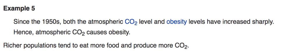
If we regress obesity on CO2 levels, we’ll likely get a positive coefficient (there are issues with the temporal structure but let’s ignore those for now). However, if we include the wealth of the population as a feature, the effect is likely to disappear. Thus the omitted variable likely leads to overestimation of the effect we originally estimated.

Let’s look at this mathematically (example is from Coursera’s econometrics course). Say we have two features $x_1$ and $x_2$ and the true model is

(3) $\begin{align*}y=\beta_1x_1+\beta_2x_2+\eta\end{align*}$

Now assume we ignore $x_2$ and regress $y=\beta_1x_1+\epsilon$ , then if $x_1$ is correlated with $x_2$ and $\beta_2\neq 0$ , we have that

(4) $\begin{align*}\textrm{Cov}(x_1,\epsilon)&=\textrm{Cov}(x_1,\beta_2 x_2+\eta)\\&=\textrm{Cov}(x_1,x_2)\beta_2+\textrm{Cov}(x_1,\eta)\\&\neq 0\end{align*}$

and thus we have endogeneity. Note that in this case, endogeneity is actually caused by model misspecification.

Measurement Error

Another cause of endogeneity is measurement error. Let’s say that $y$ is the treatment effect but we can’t accurately measure the dosage $x$ , and instead observe $x^*=x+u$ , where $u$ is some mean-zero random variable, and we fit $y=\beta x^*+\epsilon$ . In this case we will have endogeneity and OLS loses its consistency properties.

How Do We Deal With This?

If we wish to recover a consistent estimate of the parameters $\beta$ , then we need to study instrumental variables. We will discuss these in a future post.