Feedforward Neural Networks and Multilayer Perceptrons

In this post we describe multilayer perceptrons. We first describe why we want to use neural networks, and what feedforward neural networks and neurons are. Then we define multilayer perceptrons. We discuss when you should use a multilayer perceptron and how to choose an architecture. We then show an example where we apply a multilayer perceptron to the MNIST dataset.

Why Use Neural Networks?

Classical machine learning techniques such as SVMs, random forests, and KNN work well in prediction with structured data where the inputs have a clear meaning. However, for unstructured data such as images, raw speech waveforms, or wearable sensor data, plugging in the raw data into classical models tends not to work very well.

Previous solutions involved handcrafting features from the raw data: examples in computer vision include SIFT and HOG. For wearable sensors, say you’re trying to do time series classification using your sensor data. You might use a fixed sliding window and then take summary statistics, such as the mean, median, mode, and variance, over that sliding window, and then use them in a classifier. However, how do you know that those are actually the summaries of your data that are most relevant to your classification problem? In fact you rarely do. Neural networks do ‘feature learning:’ where the summaries are learned rather than specified by the data analyst.

Feedforward Neural Networks

A feedforward neural network involves sequential layers of function compositions. Each layer outputs a set of vectors that serve as input to the next layer, which is a set of functions. There are three types of layers:

Input layer: the raw input data
Hidden layer(s): sequences of sets of functions to apply to either inputs or outputs of previous hidden layers
Output layer: final function or set of functions.

Let’s look at a visual example.

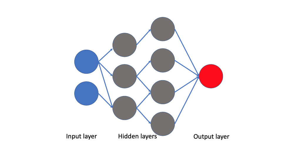
Here the blue nodes (circles) serve as the input layer: the raw data. The gray nodes or ‘neurons’ together form the hidden layers: each node takes as input the nodes from the previous layer that are connected to it, and outputs some value. The red node forms the output layer which is a final function.

One way to think about this is that the output layer is the final model that takes the last hidden layer as input. All other hidden layers are learning and then refining features of the raw inputs.

What is a Neuron?

A neuron is a single function which takes inputs and applies an activation function. The gray and red nodes in the previous image were neurons. Here is another example:

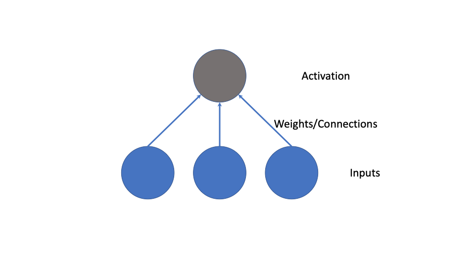
Simple examples of ‘neurons’ include the linear and logistic regression models. A vector $x$ forms the inputs, the weights are the $\beta$ values of the linear predictor, and the activation function is the identity function for linear regression and the logistic or sigmoid function for logistic regression. Thus under sigmoid activation functions, a feedforward neural network can be thought of as a ‘network’ of logistic regressions.

If are input vector is $x$ and our weight vector is $w$ , and our activation function is $f$ , then the neuron $h$ takes values as follows

(1) $\begin{align*}h&=f(w^T x)\end{align*}$

What is a Multilayer Perceptron?

A multilayer perceptron is a special case of a feedforward neural network where every layer is a fully connected layer, and in some definitions the number of nodes in each layer is the same. Further, in many definitions the activation function across hidden layers is the same. The following image shows what this means

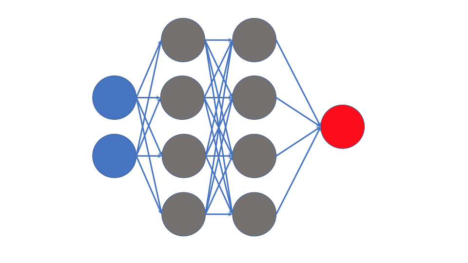
As one can see, each layer that feeds into the next connects to all nodes in the next layer.

When Should You Use a Multilayer Perceptron?

One should generally use the multilayer perceptron when one knows very little about the structure of the problem. As we mentioned previously, one uses neural networks to do feature learning. Using fully connected layers only, which defines an MLP, is a way of learning structure rather than imposing it. While one can increase the depth and width of the network, that simply increases the flexibility in function approximation. Features are entirely learned.

Later models such as convolutional neural networks are in some ways a hybrid: features are learned, but they specify the structure that relationships between pixels that are close to each other are important, while relationships between pixels further apart are not. For some problems like image classification, specifying such a structure improves prediction accuracy.

How do you Choose the Architecture?

Traditionally there were various heuristics for choosing the number of hidden layers and nodes per hidden layer. One might keep adding layers or keep adding hidden nodes and checking validation set performance. Recently [1] gives theoretical guarantees on how well a function can be approximated with an MLP with a RELU activation function under loss functions obeying certain technical conditions. Based on their theory, under certain smoothness conditions on the true function, if $n$ is our sample size, $d$ is the dimension of our input vector, and $\beta$ is a smoothness parameter, we can choose our width to be of order $n^{d/(2(\beta+d))}\log^2 n$ and depth to be of order $\log n$ . Then the function error will go to $0$ as the sample size goes to infinity with high probability. Since $\beta$ is unknown we can treat it as a hyperparameter and choose the hyperparameter that does best on a validation set.

They do not claim that this theory is optimal, but it at least gives a theoretically grounded starting point for choosing the architecture.

Example: MNIST

MNIST is a dataset of 60,000 training images and 10,000 test images of digits 0-9: the goal is to classify them. We will fit an MLP to them, following the code of https://www.tensorflow.org/tutorials/quickstart/beginner but changing the architecture based on the theory of [1]. We choose $\log(1000)\approx 11$ hidden layers. We set $\beta=100000$ and based on that use $126$ nodes. We’ll assume that the technical conditions hold for both our true function and the loss function. Copying their code except the architecture modification, we obtain

import tensorflow as tf
import numpy as np

mnist = tf.keras.datasets.mnist

(x_train, y_train), (x_test, y_test) = mnist.load_data()
x_train, x_test = x_train / 255.0, x_test / 255.0

n=60000
d=784
beta=5000
width = int(np.floor(n**(d/(2*(beta+d)))*(np.log(n)**2)))

#this part is different from the Google tutorial
model = tf.keras.models.Sequential([
  tf.keras.layers.Flatten(input_shape=(28, 28)),
  tf.keras.layers.Dense(width, activation='relu'),
  tf.keras.layers.Dense(width, activation='relu'),
  tf.keras.layers.Dense(width, activation='relu'),
  tf.keras.layers.Dense(width, activation='relu'),
  tf.keras.layers.Dense(width, activation='relu'),
  tf.keras.layers.Dense(width, activation='relu'),
  tf.keras.layers.Dense(width, activation='relu'),
  tf.keras.layers.Dense(width, activation='relu'),
  tf.keras.layers.Dense(width, activation='relu'),
  tf.keras.layers.Dense(width, activation='relu'),
  tf.keras.layers.Dense(width, activation='relu'),
])

predictions = model(x_train[:1]).numpy()
loss_fn = tf.keras.losses.SparseCategoricalCrossentropy(from_logits=True)

model.compile(optimizer='adam',
              loss=loss_fn,
              metrics=['accuracy'])
model.fit(x_train, y_train, epochs=5)
model.evaluate(x_test,  y_test, verbose=2)

Running this code gives us

Train on 60000 samples
Epoch 1/5
60000/60000 [==============================] - 8s 131us/sample - loss: 1.4537 - accuracy: 0.7025
Epoch 2/5
60000/60000 [==============================] - 7s 119us/sample - loss: 1.1218 - accuracy: 0.7702
Epoch 3/5
60000/60000 [==============================] - 7s 121us/sample - loss: 1.1027 - accuracy: 0.7738
Epoch 4/5
60000/60000 [==============================] - 8s 137us/sample - loss: 1.0745 - accuracy: 0.7795
Epoch 5/5
60000/60000 [==============================] - 8s 126us/sample - loss: 1.0621 - accuracy: 0.7821

10000/10000 - 1s - loss: 1.0656 - accuracy: 0.7840

This performance is horrible for MNIST! Most methods see accuracy in the high 90s. However, to make the comparison fare to the other tutorial, we should also use dropout like they did. We add dropout as follows.

model = tf.keras.models.Sequential([
  tf.keras.layers.Flatten(input_shape=(28, 28)),
  tf.keras.layers.Dense(width, activation='relu'),
  tf.keras.layers.Dense(width, activation='relu'),
  tf.keras.layers.Dense(width, activation='relu'),
  tf.keras.layers.Dense(width, activation='relu'),
  tf.keras.layers.Dense(width, activation='relu'),
  tf.keras.layers.Dense(width, activation='relu'),
  tf.keras.layers.Dense(width, activation='relu'),
  tf.keras.layers.Dense(width, activation='relu'),
  tf.keras.layers.Dense(width, activation='relu'),
  tf.keras.layers.Dense(width, activation='relu'),
  tf.keras.layers.Dropout(0.2),
  tf.keras.layers.Dense(width, activation='relu')
])

Running the rest of the code again with the dropout added gives us

10000/10000 - 1s - loss: 0.1237 - accuracy: 0.9697

about 97% accuracy, which is similar to the ~98% reported by the Google tutorial. The advantage we have is that thanks to theory, we didn’t need to think hard about the architecture: only our choice of $\beta$ which affects the architecture.

[1] Farrell, Max H., Tengyuan Liang, and Sanjog Misra. “Deep Neural Networks for Estimation and Inference.” arXiv preprint arXiv:1809.09953 (2018).