Gradient Descent and Momentum: The Heavy Ball Method

Contents hide

In this post we describe the use of momentum to speed up gradient descent. We first describe the intuition for pathological curvature, and then briefly review gradient descent. Next we show the problems associated with applying gradient descent to the toy example $f(x)=x^4$ . We describe how momentum, guiding the current step slightly towards the direction of the previous step, can help address these problems. Then we show improved convergence on the same example. We conclude with discussion.

A key issue in gradient descent is pathological curvature. Curvature describes how different a function is from linear, and can vary both in regions of parameter space and in different directions for a given point. When curvature in different regions and/or directions is very different, for a fixed learning rate gradient descent will make slow progress in one of either the high or low curvature regions/directions. Particularly, a large learning rate will cause gradient descent to make faster progress in regions of low curvature. However it may oscillate in regions of high curvature when a function has walls. In contrast, a small learning rate will cause gradient descent to make faster progress in regions of high curvature, but lead to small steps in regions of low curvature.

Before we continue, recall the classic gradient descent setting. Let $f:\mathbb{R}^n\rightarrow \mathbb{R}$ be a convex function with a unique minimum. Also let $x_t$ be our current estimate of its minimum. Gradient descent updates $x_t$ by noting that the gradient gives the direction of greatest increase of the function, and thus to minimize the function we should move in the opposite direction. It uses the following update rule

(1) $\begin{align*}x_{t+1}=x_t-\alpha \nabla f(x_t)\end{align*}$

where $\alpha$ is the learning rate and $\nabla f(x_t)$ is the gradient. For a one-dimensional function, the second derivative describes the curvature. In more complex settings the curvature is described by the eigenvalues of the Hessian. Eigenvectors with large magnitude eigenvalues describe directions of high curvature, and eigenvectors with small magnitude eigenvalues describe directions of low curvature.

A Toy Example: Quartic Function

The function $f(x)=x^4$ has very different curvature in different regions of data: we will see that a large learning rate leads to bigger steps than we would like in high curvature regions, while a small learning rate leads to smaller steps than we would like in low curvature regions. It has second derivative $f''(x)=12x^2$ : the curvature approaches $0$ as $x\rightarrow 0$ , and approaches $\infty$ as $|x|\rightarrow\infty$ .

Initialize $x=0.5$ and let $\alpha=1.999999999999999$ . This is about as large as $\alpha$ can be without either diverging or bouncing back and forth between $x=0.5$ and $x=-0.5$ . This gives us

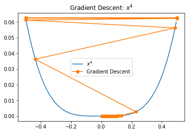
We see that we bounce along the walls of the function for some iterations, making bigger steps than we would like. While in the particular case the amount of bouncing is not large, this bouncing across walls in regions of high curvature is a common issue for gradient descent in higher dimensions. We could potentially reduce this bouncing by lowering the learning rate. If we set it to $\alpha=0.5$ , we obtain

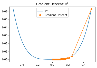
We no longer bounce along the walls and make fast progress in the region of high curvature, but then in the region of low curvature we drastically increase the number of iterations required due to very small steps towards the optimum.

Momentum

Based on the above results, we want two things:

To make smaller steps in regions of high curvature to dampen oscillations.
To make larger steps and accelerate in regions of low curvature.

One way to do both is to guide the next steps towards the previous direction. We can achieve this via a simple tweak to the gradient descent update rule

(2) $\begin{align*}x_{t+1}=x_t-\alpha\nabla f(x_t)+\underbrace{\beta(x_t-x_{t-1})}_{\textrm{momentum}}\end{align*}$

This idea comes from Polyak [1], and is also called the heavy ball method. Intuitively, a heavier ball will bounce less and move faster through regions of low curvature than a lighter ball due to momentum. This has two effects, related to the two goals stated:

We penalize changes in direction to take smaller steps
When the direction doesn’t change we take bigger steps

Quartic Example with Momentum

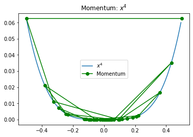
Let’s first apply momentum in the setting where we bounced across the walls. We set $\beta=0.825$ . Because the momentum update does not necessarily monotonically decrease the objective function, it is sometimes difficult to tell what’s going on from looking at plots similar to those we made above.

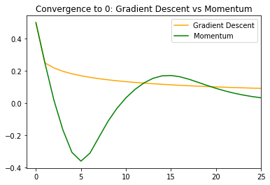
However since we know that the true minimum for this function is $x=0$ , we can plot the convergence of $x_t$ to that value. We first plot the first 25 iterations to ‘zoom in.’

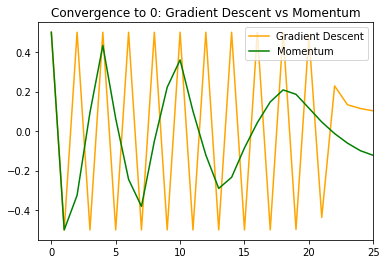
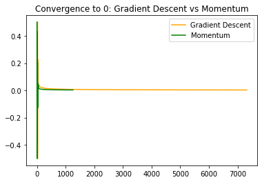
We can see that momentum leads to less bouncing across the walls, and to smaller bounces. It dampens the oscillations, making changes in direction involve smaller steps and leading to fewer changes in direction. This gets us closer to the true value more quickly. If we zoom out and plot the entire convergence, we see

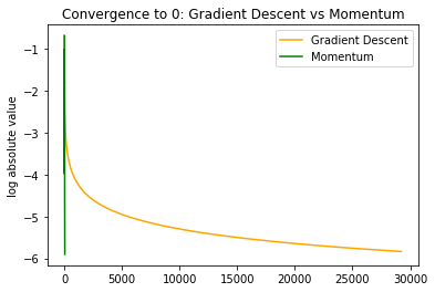
and in log scale for the absolute value we see

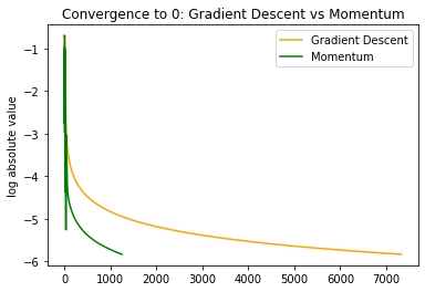
thus not only are oscillations dampened, but we also make much faster progress in the regions of low curvature when $x$ is already close to $0$ .

Next we can look at the example with the smaller learning rate of $\alpha=0.5$ . We set $\beta=0.8$ . We can make the same ‘zoomed in’ convergence to $0$ plot

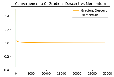
interestingly in this case momentum has some oscillation that isn’t there in naive gradient descent, although the oscillation is mild. Zooming back out we can see that momentum has drastically faster convergence. This is due to poor progress of gradient descent in the region of low curvature.

Discussion

In this post we described momentum. We first described the issue of different curvature in different regions of data. Next we shows how this affects learning for the simple function $f(x)=x^4$ . We used the issues found to motivate momentum: nudging the current update in the direction of the previous update. We show how this improves learning $f(x)=x^4$ .

[1] Polyak, Boris T. “Some methods of speeding up the convergence of iteration methods.” USSR Computational Mathematics and Mathematical Physics 4, no. 5 (1964): 1-17.

A Toy Example: Quartic Function

Momentum

Quartic Example with Momentum

Discussion

Related Posts

Leave a Reply Cancel reply