Stationarity and Non-stationary Time Series with Applications in R

Contents hide

1 Background

1.1 Why Stationarity?

1.2 What is Stationarity?

1.3 Weak Sense Stationarity

2 Non-Stationarity

2.1 Trend Stationarity

In this post we describe stationary and non-stationary time series. We first ask why we want stationarity, then describe stationarity and weak sense stationarity. Next we discuss trend stationarity and the KPSS test. We finish with a discussion of stochastic trends and differencing.

Background

Why Stationarity?

In time series analysis, we’d like to model the evolution of a time series $\{x_t\}_{t=0}^\infty$

from observations $x_0,x_1,\cdots,x_T$

. We particularly want to model moment functions of the time series. For instance, the mean function describes how the average value evolves over time, while the conditional mean function describes the same given past values. The autocovariance function describes the covariance between values at different points in time. We may also be interested in higher moment functions. When estimating parameters describing these, we’d like to be able to apply standard results from probability and statistics such as the law of large numbers and the central limit theorem.

If the moment functions are constant, then that greatly simplifies modeling. For instance, if the mean is $\mu$

instead of $\mu(t)$

then we estimate a constant rather than a function. This applies similarly to higher moments.

What is Stationarity?

A stochastic process $x_0,x_1,\cdots$

is stationary if for any fixed $p\in \mathbb{N},p(x_t,\cdots,x_{t+p})$

does not change as a function of $t$

. In particular, moments and joint moments are constant. This can be described intuitively in two ways: 1) statistical properties do not change over time 2) sliding windows of the same size have the same distribution.

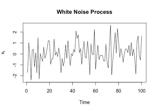
A simple example of a stationary process is a Gaussian white noise process, where each observation $x_t$

is iid $\mathcal{N}(0,\sigma^2)$

. Let’s simulate Gaussian white noise and plot it: many stationary time series look somewhat similar to this when plotted.

white_noise<-rnorm(100,0,1)
plot(white_noise,type='l',xlab='Time',ylab=expression('x'[t]),main='White Noise Process')

A simple example of a non-stationary process is a random walk. This is a sum of iid random variables with mean $0$

. Let’s use rademacher random variables (take values $\pm 1$

each with probability $0.5$

). We’ll simulate $10,000$

steps and plot it.

library(extraDistr)
random_walk<-cumsum(rsign(10000))
plot(random_walk,type='l',xlab='Time',ylab=expression('x'[t]),main='Random Walk')

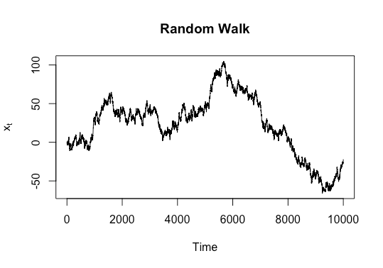
It’s not super easy to see this from plots, but it can be shown mathematically that the variance of the time series increases over time, which violates stationarity.

Weak Sense Stationarity

Often we are primarily interested in the first two moments of a time series: the mean and the autocovariance function. A process is weak sense or weakly stationary if

(1) $\begin{align*}\mu(t)&=\mathbb{E}x_t=\mu\\\textrm{Cov}(X_t,X_s)&=\textrm{Cov}(X_{t-s},X_0)\forall t>s\in \mathbb{N}\end{align*}$

That is, if the mean does not depend on time and the autocovariance between two elements only depends on the time between them and not the time of the first. An important motivation for this is Wold’s theorem. This states that any weakly stationary process can be decomposed into two terms: a moving average and a deterministic process. Thus for a purely non-deterministic process we can approximate it with an ARMA process, the most popular time series model. Thus for a weakly stationary process we can use ARMA models. Intuitively, if a process is not weakly stationary, the parameters of the ARMA models will not be constant, and thus a constant model will not be valid.

Non-Stationarity

Non-stationarity refers to any violation of the original assumption, but we’re particularly interested in the case where weak stationarity is violated. There are two standard ways of addressing it:

Assume that the non-stationarity component of the time series is deterministic, and model it explicitly and separately. This is the setting of a trend stationary model, where one assumes that the model is stationary other than the trend or mean function.
Transform the data so that it is stationary. An example is differencing.

Trend Stationarity

A trend stationary stochastic process decomposes as

(2) $\begin{align*}x_t&=\mu_t+y_t\end{align*}$

Here $\mu_t$

is the deterministic mean function or trend and $y_t$

is a stationary stochastic process. An important issue is that we need to specify a model for the mean function $\mu_t$

: generally we use a linear trend, possibly after a transformation (such as $\log$

Assuming that we know that trend stationarity holds, we do a three step process:

Fit a model $\hat{\mu}_t$ to $x_t$
Subtract $\hat{\mu}_t$ from $x_t$ , obtaining $\hat{y}_t=x_t-\hat{\mu}_t$
Model $\hat{y}_t$ (inference, forecasting, etc)

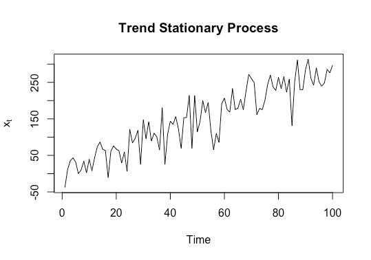
Let’s look at a synthetic example of a trend stationary process $x_t=3t+\epsilon_t$

where $\epsilon_t$

is $\mathcal{N}(0,40)$

white noise. We can generate and plot this via the following code:

white_noise<-rnorm(100,0,40)
trend<-3*(1:100)
x_t<-trend+white_noise
plot(x_t,type='l',xlab='Time',ylab=expression('x'[t]),main='Trend Stationary Process')

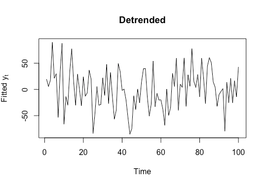
We can then detrend and plot the detrended series

mu_t<-lm(x_t~c(1:100))
y_t<-x_t-mu_t[['fitted.values']]
plot(y_t,type='l',xlab='Time',ylab=expression('Fitted y'[t]),main='Detrended')

The KPSS Test

With real data where we don’t know if trend stationarity holds, we need a way to test it. We can use the KPSS test [1]. This assumes the following model specification:

(3) $\begin{align*}x_t&=\alpha+\beta t+u_t+y_t\end{align*}$

Here $u_t$

is a random walk with $\mathcal{N}(0,\sigma^2_u)$

increments and $y_t$

is a stationary process. We are interested in the following null and alternate hypotheses:

$H_0$

: $\sigma_u=0$

$H_1$

: $\sigma_u>0$

Under the null, $x_t$

is trend stationary with $\mu_t=\alpha+\beta t$

since the random walk disappears. Let’s look at an example of US log gross national product (GNP). Before running the test, let’s plot the original and detrended series.

data<-USeconomic[,'log(GNP)']
fit <- lm(data~time(data), na.action=NULL)
plot(data,main='Log GNP',ylab='log(GNP)')
resid<-data-fit[['fitted.values']]
plot(resid,main='Detrended Log GNP',ylab='Detrended log(GNP)')

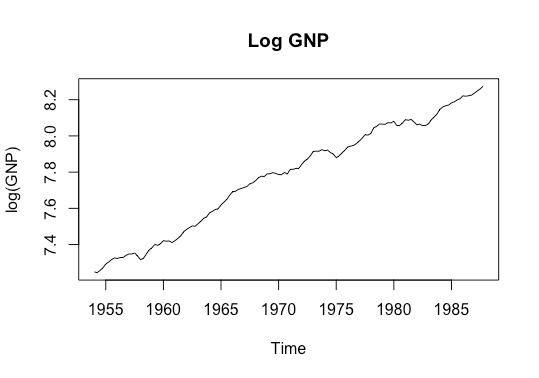
This plot looks quite linear, so perhaps it is trend stationary. Let’s look at the detrended series.

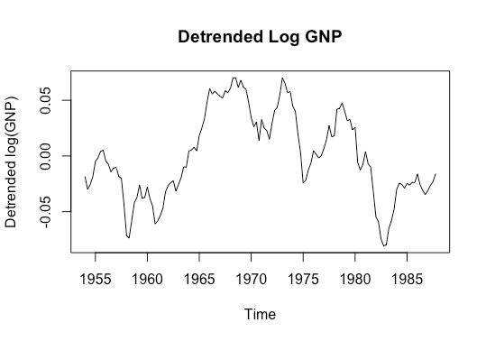
It looks from the second plot like the detrended series still has a non-linear mean, suggesting that the true trend may not be linear. Let’s run a KPSS test on the original series.

kpss.test(data,'Trend')

p-value smaller than printed p-value
	KPSS Test for Trend Stationarity

data:  data
KPSS Trend = 0.44816, Truncation lag parameter = 4, p-value = 0.01

We thus reject the null hypothesis of trend stationarity. In fact, if you try running the KPSS test for various time series datasets shown by the command data() in R, you won’t find many (I believe any although I may have missed something) that fail to reject the null hypothesis. Trend stationarity is fairly rare in practice. Further, even if trend stationarity does hold, it requires correct model specification for the trend: if the trend is non-linear this can be difficult.

This motivates finding another approach.

Differencing

Stochastic Trend

One possibly more realistic model is that described by the alternate hypothesis of the KPSS test: $x_t=\alpha+\beta t+u_t+y_t$

, where $u_t$

is a Gaussian random walk and $y_t$

is a stationary process. We then call $\alpha+\beta t +u_t$

the stochastic trend: this describes both the deterministic mean function and shocks that have a permanent effect. While this is a more realistic model than the trend stationary model, we need to extract a stationary time series from $x_t$

Differencing

One way to do this is via differencing: that is, to take $\nabla x_t=x_t-x_{t-1}$

. For the trend stationary model, the difference process is stationary. We then say that $x_t$

is a difference stationary process. Intuitively one can think of differencing as similar to differentiation in calculus. One can keep ‘differentiating’ (differencing) until one has removed the dependence on $t$

from the mean and variance, leading to a weakly stationary process. For example consider a process $x_t$

such that $\mathbb{E}x_t=t^2$

. Then $\mathbb{E}\nabla x_t=2t-1$

, lowering the order of the polynomial. Doing this again gives $\mathbb{E}\nabla\nabla x_t=0$

, which is constant.

Let’s look at the differenced log GNP data.

plot(diff(data),ylab='diff(log(GNP))', main='Differenced Log GNP')

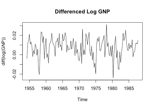
There isn’t any obvious non-stationary: the mean doesn’t seem time-varying, nor does the auto-covariance function, although the latter is harder to inspect visually. We can also do an augmented Dickey Fuller test, with the alternate hypothesis of no unit root (a unit root would imply non-stationarity).

adf.test(diff(data))

Augmented Dickey-Fuller Test

data:  diff(data)
Dickey-Fuller = -4.4101, Lag order = 5, p-value = 0.01
alternative hypothesis: stationary

Thus we reject the null hypothesis of a unit root.

Discussion

In this post, we describe the concepts of stationary and non-stationary time series. We discuss the definitions, weak sense stationarity, trend stationarity and the KPSS test, stochastic trends, and differencing.

[1] Kwiatkowski, Denis, Peter CB Phillips, Peter Schmidt, and Yongcheol Shin. “Testing the null hypothesis of stationarity against the alternative of a unit root.” Journal of econometrics 54, no. 1-3 (1992): 159-178.

Background

Why Stationarity?

What is Stationarity?

Weak Sense Stationarity

Non-Stationarity

Trend Stationarity

The KPSS Test

Differencing

Stochastic Trend

Differencing

Discussion

Related Posts

Leave a Reply Cancel reply