An Introduction to Time Series Smoothing in R

Contents hide

In this post we describe the basics of time series smoothing in R. We first describe why to do smoothing, then describe the simple moving average and how it performs poorly on very noisy data, then describe the triangular moving average and the kernel smoother, which often perform better on high noise data.

Why do Smoothing?

Time series modeling has several potential goals. These include inference, where we want to describe how the stochastic process evolves, forecasting, where we want to predict the future, and classification, where we want to classify a subsequence of a time series. All of these rely on capturing at least one of either the low frequency or the high frequency behavior in order to achieve the goal successfully.

A time series can generally be decomposed into several components: trend, cyclical, seasonal, and noise. These are in order of increasing frequency. As a blog owner, one way I see these is as follows. Noise is simply the random variation in daily views. The seasonal component is that there are fewer viewers on the weekends. The cyclical is that Google’s algorithms cause readership to go up and down, and the trend is that over time, readership tends to go up.

Smoothing attempts to progressively remove the higher frequency behavior to make it easier to describe the lower frequency behavior. Ideally, a small amount of smoothing removes noise, more smoothing removes the seasonal component, and then finally the cyclical component is removed to isolate trend. Bad smoothers for a given dataset often remove more than one component at a time: for instance, they may not be able to smooth out noise without smoothing out seasonality. In the next sections we describe some smoothers and apply them to standards R datasets.

Smoothers

Simple Moving Average

The simplest smoother is the simple moving average. Assume we have a time series $x_1,\cdots,x_T$ . Then for each subsequence $x_i,\cdots,x_p$ , compute

(1) $\begin{align*}\tilde{x}_i&=\frac{1}{p}\sum_{k=l}^{l+p}x_k\end{align*}$

where $l\leq i$ and $l$ controls the alignment of the moving average. Here $p$ is called the filter size or window. Let’s look at an example to see how smoothing works in practice. We’ll start with a moderately low noise dataset, the R AirPassengers dataset, with the monthly airline passenger numbers from 1949-1960. We’ll plot the original dataset, a simple moving average with filter size $10$ , and one with filter size $40$ .

data<-AirPassengers
plot(data,main='Simple Moving Average (SMA)',ylab='Passengers')
lines(rollmean(data,5),col='blue')
lines(rollmean(data,40),col='red')
legend(1950,600,col=c('black','blue', 'red'),legend=c('Raw', 'SMA 5', 'SMA 40'),lty=1,cex=0.8)

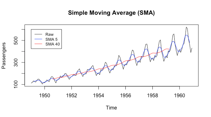
From the plot we can see that the black curve has some jagged parts, which tend to repeat themselves. We may want to smooth them out to get a ‘high level summary’ of the seasonal component. The blue curve gives that to us. The red curve, with a larger filter size, focuses more on the trend. The simple moving average seems to do a good job at different levels of smoothing.

Now let’s look at a higher noise dataset, the R discoveries dataset. This describes the number of ‘great’ discoveries and inventions from 1860 to 1959. Let’s plot the raw data along with simple moving averages with filter sizes $5$ and $10$ , respectively.

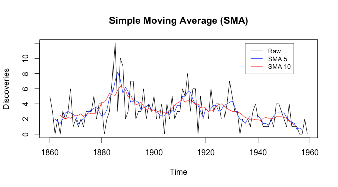
Firstly we see that the raw data is very noisy. Secondly, we see that both the simple moving averages are still fairly noisy, despite the red having much smaller local peaks. There doesn’t seem to be a seasonal component, but there is a cyclical component, and there is likely no trend. It appears that in this setting in order to smooth out noise one also smooths out much of the cyclical component. Is there some way to smooth out noise while keeping more of the cyclical and seasonal components in these very noisy datasets?

Triangular Moving Average

One method that works fairly well for this is the triangular moving average: this is simply a moving average applied twice. Let’s plot two simple moving averages with filter size $5$ and $10$ , respectively, and one triangular moving average (denoted TMA) with filter size $5$ .

p=5
plot(rollmean(data,p),main='Simple vs Triangular Moving Average',ylab='Discoveries')
lines(rollmean(data,10),col='red')
lines(rollmean(rollmean(data,5),5),col='blue')
legend(1935,8,col=c('black','red','blue'),legend=c('SMA 5', 'SMA 10','TMA 5'),lty=1,cex=0.8)

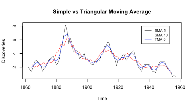
We can see that the triangular moving average is smoother and has less noise than both of the simple moving averages, but keeps more of the peaks than the simple moving average with filter size $10$ .

Kernel Smoothing

Another method that works fairly well for noisy datasets is kernel smoothing. This takes a weighted average over the entire observed data, where the weights are determined by a kernel function, with hyperparameters set by the data analyst to control the amount of smoothness. Intuitively, the weights are some non-linear function of the distance between the current time and the time associated with the observation being weighted. We then have

(2) $\begin{align*}\tilde{x}_t&=\frac{\sum_{i=1}^nK(t,i)x_i}{\sum_{j=1}^N K(t,i)}\end{align*}$

A popular choice of Kernel is the Gaussian Kernel. Here

(3) $\begin{align*}K(t,i)&=\exp(-\frac{(t-i)^2}{2b^2})\end{align*}$

where we call $b$ the bandwidth. This is a type of exponential decay. Let’s plot kernel weights as a function of distance from the current point for different bandwidths.

last_point = 100
b=1
plot(0.1*0:last_point,exp(-(0.1*0:last_point)^2/(2*b^2)),type='l',xlab='distance',ylab='weight',main='Gaussian Kernel Weights')
b=2
lines(0.1*0:last_point,exp(-(0.1*0:last_point)^2/(2*b^2)),type='l',col='red')
b=5
lines(0.1*0:last_point,exp(-(0.1*0:last_point)^2/(2*b^2)),type='l',col='blue')
legend(7,1,legend=c('b=1','b=2','b=5'),col=c('black','red','blue'),cex=0.8,lty=1)

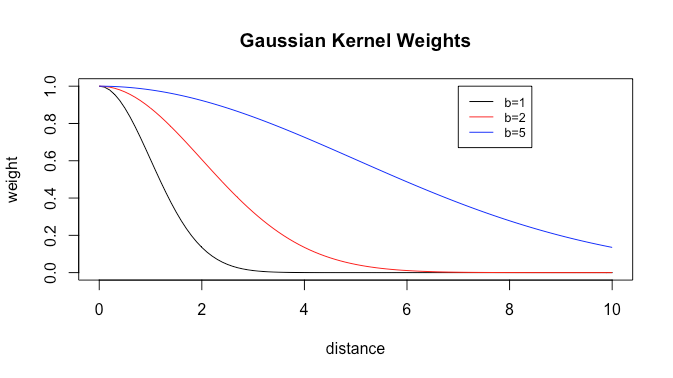
We see that the greater the bandwidth, the slower the weight decay, and thus the more weights there are that are not (very close to) zero. Thus greater bandwidth gives more smoothing. Now let’s try plotting simple moving averages of filter size $5$ and $10$ against Gaussian kernel smoothing with $b=4$ .

p=5
b=4
plot(rollmean(data,p),main='Simple Moving Average vs Kernel Smoothing',ylab='Discoveries')
lines(rollmean(data,10),col='red')
lines(ksmooth(time(data),data,'normal',bandwidth=b),type='l',col='blue')
legend(1935,8,col=c('black','red','blue'),legend=c('SMA 5', 'SMA 10', 'Kernel,b=4'),lty=1,cex=0.8)

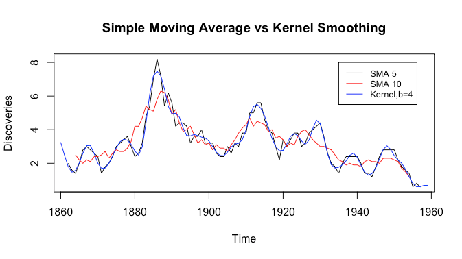
Like the triangular moving average, we see that the kernel smoother is smoother than both simple moving averages, while keeping the peaks that the simple moving average with filter size $10$ smooths out. Let’s now try comparing the triangular moving average with kernel smoothing.

plot(rollmean(rollmean(data,5),5),main='Triangular Moving Average vs Kernel Smoothing',ylab='Discoveries')
lines(ksmooth(time(data),data,'normal',bandwidth=b),type='l',col='blue')
legend(1935,6,col=c('black','blue'),legend=c('TMA 5','Kernel b=4'),lty=1,cex=0.8)

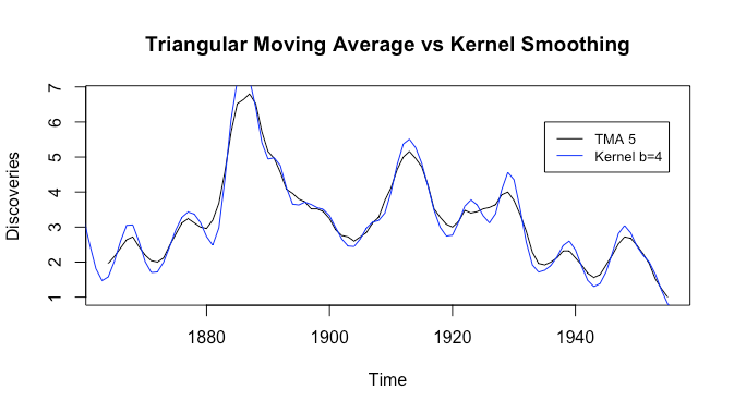
It’s a bit hard to compare: what if we change the bandwidth to $6$ ?

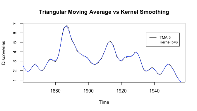
Now they look almost identical, although the kernel smoother seems slightly smoother.

Choosing a Smoother

We’ve seen some smoothers, but for a given dataset, how do we choose a smoother, and how do you choose hyperparameters? A first thing to note is that for low noise time series, many given smoothers can be made to give very similar results for the appropriate choice of hyperparameters (filter size, bandwidth in the kernel setting, etc). Thus it often makes sense to use a simple moving average in the low noise case. As noise levels increase, one needs to think more carefully about what else you’ll smooth out along with noise when using different smoothers: some experimentation along with visualization is recommended.

The second question should be: what is your problem, and what components do you need to isolate for that problem? If you’re trying to do forecasting, potentially you want to capture all of trend, cyclical, and seasonal behavior. When doing inference on trend, you might only need to capture trend. If you’re trying to do visualization, you might want to progressively smooth each component out until only trend remains.

Discussion

In this post we discussed smoothing a time series. We discussed why you want to smooth a time series, three techniques for doing so, and how to choose a smoother.

2 Replies to “An Introduction to Time Series Smoothing in R”

R says:
January 21, 2022 at 7:21 pm
These smoothers, with the exception of moving averages, all change past values to maintain “smoothness” when working with dynamic data. Are there any smoothers that do not change past values?
Reply
1. Alex says:
  January 22, 2022 at 5:48 pm
  Hi, I don’t fully understand the question. Firstly, what do you mean with dynamic data: do you mean that you observe the data coming in streaming fashion? Secondly, smoothing generally means replacing an observation with a linear combination (often a weighted average) of it and neighboring observations, and the smoothed time series thus has all values ‘changed:’ none remain the same as the original.
  Reply