In this post we describe the basics of 1-d convolutional neural networks, which can be used in time series forecasting and classification for fixed length windows. We describe why we want them, what their architecture looks like, and provide simulations to help understand what the early layers are doing. We focus on what the different types of layers are doing intuitively rather than how to do learning: we’ll discuss that in a later post.
Motivation
Many problems involve forecasting or classification with univariate time series data. One might want to classify activity from a sensor, some heart state of compensated or decompensated heart failure, or forecast future GDP. However, often there is a large amount of noise in the time series in addition to the signal. For instance, sensor readings are notoriously noisy and contain many patterns that are not related to what activity someone is performing.
In time series analysis, traditionally someone applies some sort of smoothing technique prior to analysis. One could apply a moving average to smooth a time series, and then apply a forecasting or classification technique after that. One might also apply a weighted moving average based on domain knowledge. However: how does one know that one chose good parameters for smoothing? Is there any way to get those weights automatically?
Convolutional Neural Networks
Convolutional neural networks provide us a ‘yes’ to the previous question, and give an architecture to learn smoothing parameters. The first two layers of a convolutional neural network are generally a convolutional layer and a pooling layer: both perform smoothing. Because they are part of the same function that outputs predictions, by optimizing the neural network loss, one optimizes smoothing parameters directly to perform well on a prediction task. The later layers then use the smoothed raw data and handle the main part of the time series forecasting or classification problem.
Architecture
A simple convolutional neural network architecture looks as follows
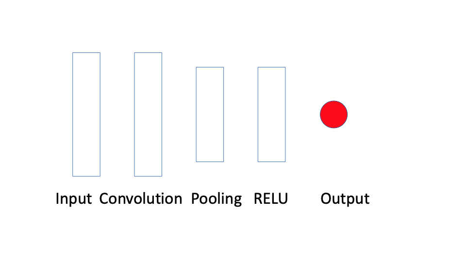
The input layer takes some a fixed length sub-sequence of the full time series and passes them to the convolutional layer. The convolutional and pooling layers, which we will describe soon, smooth the input. The RELU layer applies a RELU non-linear transformation to the smoothed sub-sequence, and the output takes the vector-valued result of that and plugs it into another activation function to give you class probabilities, a continuous-valued response, counts, or some other type of response based on the choice of activation function.
Convolutional Layers
What is a Convolution?
A convolution can be thought of a ‘weighted sum of memories’ or echoes [1,2]. To paraphrase [1], assume that  is sound and
  is the proportion one heard from
  seconds ago, and that one can only hear sound at discrete time steps. Then what you hear at time
  is
is
(1) 
Note that this is a weighted moving average, where the weights are given by the function  . Thus a discrete-time convolution generalizes a moving average so that the weights are non-zero and may not sum to
  . Like a moving average, it smooths a time series, as we shall see.
How does a Convolutional Layer Work?
A 1-d convolutional takes an input vector  and a filter
  where
where  (usually
  ). For each neighboring set of
  elements of
![\boldsymbol{x}[i:i+k]](https://boostedml.com/wp-content/ql-cache/quicklatex.com-50a40dc1f41f2e0ea281143baef7a3c9_l3.png "Rendered by QuickLaTeX.com") one takes
one takes ![w^T\boldsymbol{x}[i:i+k]](https://boostedml.com/wp-content/ql-cache/quicklatex.com-824660699977c54af23f71103fd01580_l3.png "Rendered by QuickLaTeX.com") and that gives one node of the convolutional layer. We can see this visually. Here
and that gives one node of the convolutional layer. We can see this visually. Here  and
and  . The filter here is
  and to apply this to the first three elements
  of we do
  . We then apply the same to
  , and
, and  .
.
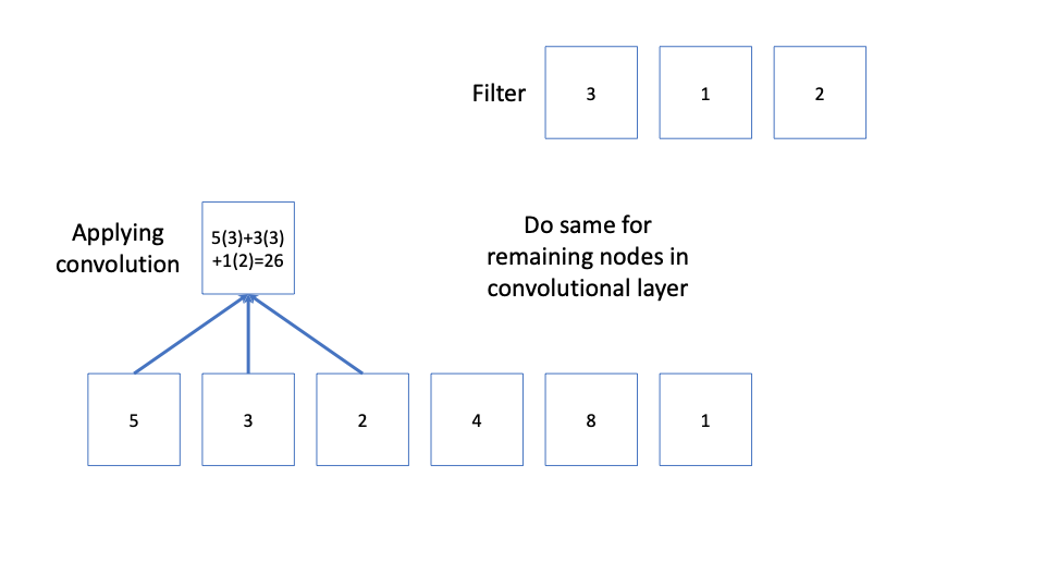
The convolution layer may have multiple filters. The vectors (one for each filter) resulting from taking all of these inner products of the weights and every elements of the original vector is the convolutional layer.
Pooling
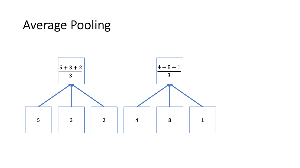
Pooling involves chunking a vector into non-overlapping equal sized groups or ‘pools’, and then taking a summary statistic for each group. This further smooths out noise in local dynamics. Three common types of pool are max pooling (very common with images), average or mean pooling, and min pooling. This image below shows average pooling.
RELU Layer
The relu layer takes the smoothed vector from applying a convolutional and pooling layer, and then applies non-linearity to it to prepare it for the final out put layer.
Output Layer
The final output layer takes a representation of our original data that has undergone two layers of smoothing and one layer of non-linear transformation, and applies an activation function to a weighted sum of that representation to output data that is of the relevant form based on our choice of activation function. This could be class probabilities, a continuous-valued response, count data, or ordinal data.
Simulation Example
Here we simulate a sequence, applying a convolution that sequence, and then apply average pooling to get some intuition for how these layers change our original data. We simulate a Gaussian random walk with  increments along with
  time steps. We then convolve this with filter
  . While there isn’t really any signal in a random walk, it can show us the smoothing idea. Here is the simulation code.
import numpy as np
import skimage.measure
from matplotlib import pyplot as plt

x=np.random.normal(0,10,100)
y=np.cumsum(x)
z=np.array([1,1,2,5,3])
y_convolved=np.convolve(y,z,mode='same')
y_convolved = np.matrix(y_convolved).T

plt.plot(y,label='original')
plt.legend()
plt.title('Gaussian Random Walk')

plt.plot(y_convolved,label='convolved')
plt.legend()
plt.title('Convolved Gaussian Random Walk')
The image below shows the original random walk and what it looks like after applying convolution.
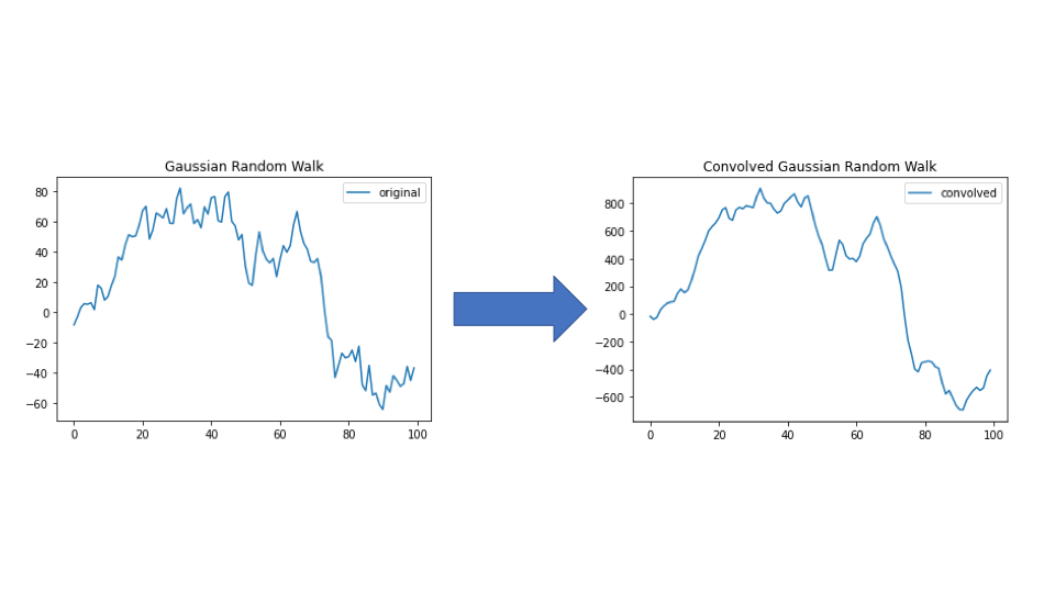
As we can see, much of the noise has been smoothed out, and the resulting plot looks far less jagged. We then apply average pooling with pools of size  . This gives us
average_pooling = skimage.measure.block_reduce(y_convolved,(3,1),np.mean)

plt.plot(average_pooling,label='average pooling')
plt.legend()
plt.title('Average Pooling of Convolved Gaussian Random Walk')
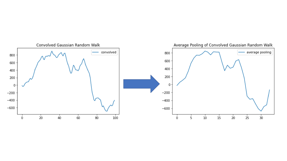
Again this is much smoother. If there was signal in this data it would be much easier to identify it in the average pooling plot than either the original random walk or the convolved random walk.
Real Data: Activity Recognition
Now let’s look at a real dataset to see if, in fact, a learned convnet does smoothing. Note this analysis is focused on investigating if a learned model smooths the time series, and is not optimized for accuracy. Discussion about accuracy will come later.
We analyze the following dataset https://archive.ics.uci.edu/ml/datasets/Activity+Recognition+from+Single+Chest-Mounted+Accelerometer. This is a dataset of seven activities performed while wearing a chest accelerometer, which has x, y, and z readings. Since we’re focused on understanding what a convnet learns, we’ll focus on x only and only use a single participant. We’ll assume that you’ve already saved the dataset in the relevant folder. Let’s load it:
participant_file_names = []
participants = []
for i in range(1,16):
    participant_file_names.append(genfromtxt('Activity Recognition from Single Chest-Mounted Accelerometer/%i.csv'%(i), delimiter=','))
    participants.append(genfromtxt('Activity Recognition from Single Chest-Mounted Accelerometer/%i.csv'%(i), delimiter=','))

participants_train = [participants[0]]
Now let’s create dataframes to hold rolling windows of accelerometer windows and the ending activity over those rolling windows.
import pandas as pd
from scipy.stats import mode
n=0
p = 50
TIME_PERIODS = p
num_sensors = 1
x = []
y = []

for k in range(len(participants_train)):
    x_participant = pd.DataFrame(participants_train[k][:,1])
    x_participant = pd.concat([x_participant.shift(i) for i in range(p)], axis=1).dropna()
    y_participant = pd.DataFrame(participants_train[k][:,4])
    y_participant = y_participant[p-1:]
    x.append(x_participant)
    y.append(y_participant)

x = np.vstack(x)
x = np.expand_dims(x,2)
y = np.hstack(y)
y = y.flatten()
We can then set our number of filters, filter size, and pool size
n_filters = 4
filter_size = 3
pool_size = 2
Now let’s specify the architecture and train for one epoch.
from tensorflow.keras.utils import to_categorical
y_binary = to_categorical(y)
tf.random.set_seed(1)
model = tf.keras.models.Sequential([
  tf.keras.layers.Reshape((TIME_PERIODS, num_sensors), input_shape=(TIME_PERIODS,num_sensors)),
  tf.keras.layers.Conv1D(n_filters, filter_size, activation='relu', padding='same',input_shape=(TIME_PERIODS, num_sensors)),#,kernel_constraint=tf.keras.constraints.NonNeg()
  tf.keras.layers.Conv1D(n_filters, filter_size, activation='relu'),
  tf.keras.layers.MaxPooling1D(pool_size),
  tf.keras.layers.Dense(100,activation='relu'),
  tf.keras.layers.Dense(y_binary.shape[1])
])

loss_fn = tf.keras.losses.CategoricalCrossentropy(from_logits=False)
adam = tf.keras.optimizers.Adam(lr=0.001, learning_rate=0.001, beta_1=0.9, beta_2=0.999, epsilon=1e-07, amsgrad=False,name='adam')
model.compile(optimizer='adam',
              loss=loss_fn,
              metrics=['accuracy'])
model.fit(x, y_binary,batch_size=64, epochs=1)

Train on 162452 samples
162452/162452 [==============================] - 30s 185us/sample - loss: 8.8828 - accuracy: 0.5153
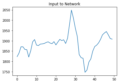
Now borrowing a function described in this https://stackoverflow.com/a/46359250/1157605, we can output intermediate layers. We start by inputting some specific window of our accelerometer readings, plotting it, and then plotting the output of the first conv layer.
from tensorflow.keras.models import Model

intermediate_layer_index = 1

intermediate_layer_model = Model(inputs=model.input,
                                 outputs=model.get_layer(index=intermediate_layer_index).output)

x_predict = np.matrix(x[50000,:,:])
x_predict = np.expand_dims(x_predict,0)
intermediate_output = intermediate_layer_model.predict(x_predict)
plt.plot(x_predict[0,:,:])
plt.title('Input to Network')
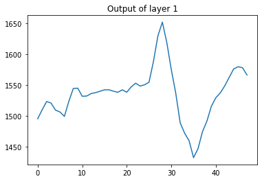
For the first conv layer we truncate the first and last point in the plot as it’s easier to visualize. We plot the output of the 2nd filter (some filters are harder to interpret as smoothing).
plt.plot(intermediate_output[0,1:49,1])
plt.title('Output of layer %i'%(intermediate_layer_index))
this was the first conv layer. We can also do the same and plot the output of the max pooling layer by changing intermediate_layer_index = 3. We plot the pool layer from the 1st filter.
plt.plot(intermediate_output[0,:,0])
plt.title('Output of layer %i'%(intermediate_layer_index))
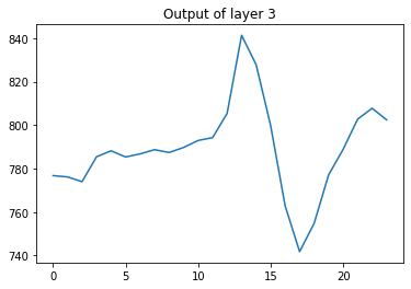
This smooths the original signal. In order to see it more closely, we plot them one after the other:
Discussion
In this post we describe what a 1-d convolutional neural network is and how the early convolutional and max pooling layers are applying smoothing to the input vector, a fixed length sub-sequence of a time series. Unlike many time series models, the convolutional neural network learns the smoothing parameters jointly with the classification or regression parameters.
[1] Ben McKay (https://mathoverflow.net/users/13268/ben-mckay), What is convolution intuitively?, URL (version: 2019-06-22)
[2] https://dsp.stackexchange.com/a/4725
Hello,
don’t you forget to Flatten after MaxPooling1D
Cz either you end up with ouput (24, 8) in final Dense
So it become :
model = Sequential([
Reshape((TIME_PERIODS, num_sensors), input_shape = (TIME_PERIODS, num_sensors)),
Conv1D(n_filters, filter_size, activation=’relu’, padding=’same’,input_shape=(TIME_PERIODS, num_sensors)),#,kernel_constraint=tf.keras.constraints.NonNeg()
Conv1D(n_filters, filter_size, activation=’relu’),
MaxPooling1D(pool_size),
Flatten(),
Dense(100, activation = ‘relu’),
Dense(y_binary.shape[1])
])