In this post we describe the basics of missing data. We first ask whether we should consider the data to truly be missing. Next, we describe the different assumptions for types of missing data. Then, we describe how missing data can appear in cross-sectional, time series, and longitudinal/panel settings. In future posts we will cover both some heuristics and principled methods for handling missing data in various settings.
Is your Data Actually Missing?
In the introduction to their book on missing data, Little and Rubin [1] identify three examples. They consider two of these examples to be missing data, and they consider one to be an additional value of that variable. The first two, the missing data examples, involve a participant who refuses to report income on a survey, and a machine that takes measurements that breaks. In both cases, there is a true underlying value that is unknown. The third example which is really another variable value, is when a participant doesn’t fill out an opinion survey about political candidate preferences because they are unsure what their opinion is. This is really a third value that lies in between the two choices.
Before deciding to treat data as missing, one should consider whether one really has missing data with some true value underlying it, or whether the seeming missingness really reflects another value of the variable.
Assumptions
There are three major assumptions for the generating process of missing data. They are:
- MCAR: missing completely at random
- MAR: missing at random
- MNAR: missing not at random
MCAR: missing completely at random
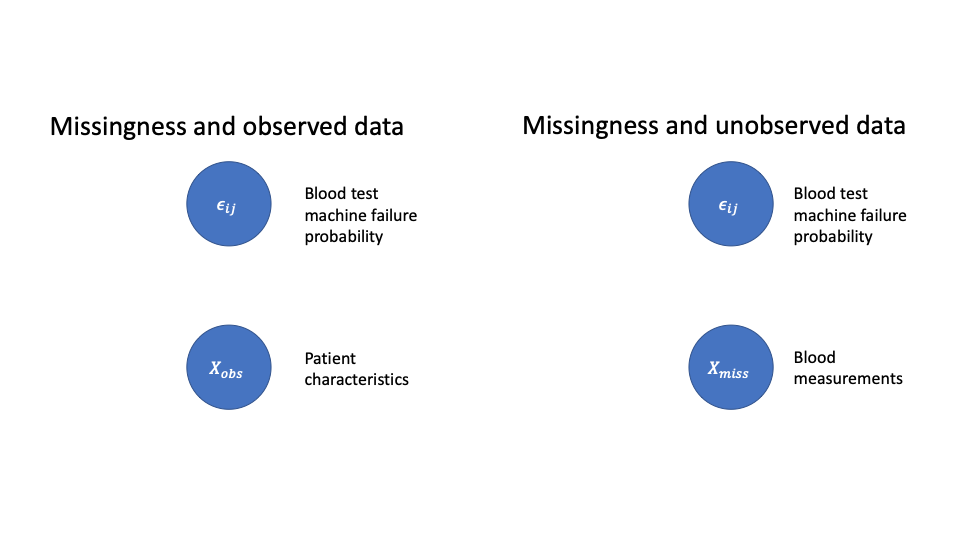
MCAR means that the missingness probability depends on neither the observed data nor the unobserved data. As an example, consider the setting of a health instrument that takes blood sample measurements from patients. Usually, the instrument failing will not be related to either the observed characteristics of the patient, or the unobserved blood measurements.
More formally, consider the cross-sectional setting where for each observation  , we have
  variables. Let
  be the complete data matrix,
  be the matrix of observed data,
  the missing data, and
  is the probability of variable
  missing from observation
  . Then the missingness is MCAR if
  and
and  , where
  indicates independence.
A graphical model representation of this assumption is below. We see that depends on neither the observed nor the unobserved data. Here the lack of any connections indicates independence.
MAR: Missing at Random
In this setting the missingness probability depends on the observed data, but not the unobserved data when conditioned on the observed data. As a cross-sectional example mentioned in wikipedia, men may be more likely to fill out a survey, but when adjusted for the fact that they are men, the missingness does not depend on the response values.
More formally, consider the same previous setting. Here the assumption is  , but
, but  . Here
  indicates dependence. Let’s look at potential graphical model representations for this assumption. There are more possible cases here. Here the arrow indicate direction of influence in the dependence structure.
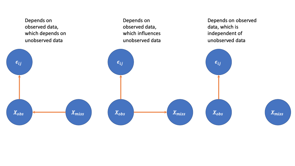
Let’s consider what each of these assumptions means in terms of the survey example. For the first one, the value of the missing data influenced the fact that you were male, which influenced the response probability for some question. That’s probably wrong for this setting, although may be correct for another. For the second, the fact that you are male influences both the missingness probability and the value of the missing data. For the third, the fact that you are male influenced the missingness probability, but is independent of the missing response values.
MNAR: Missing Not at Random
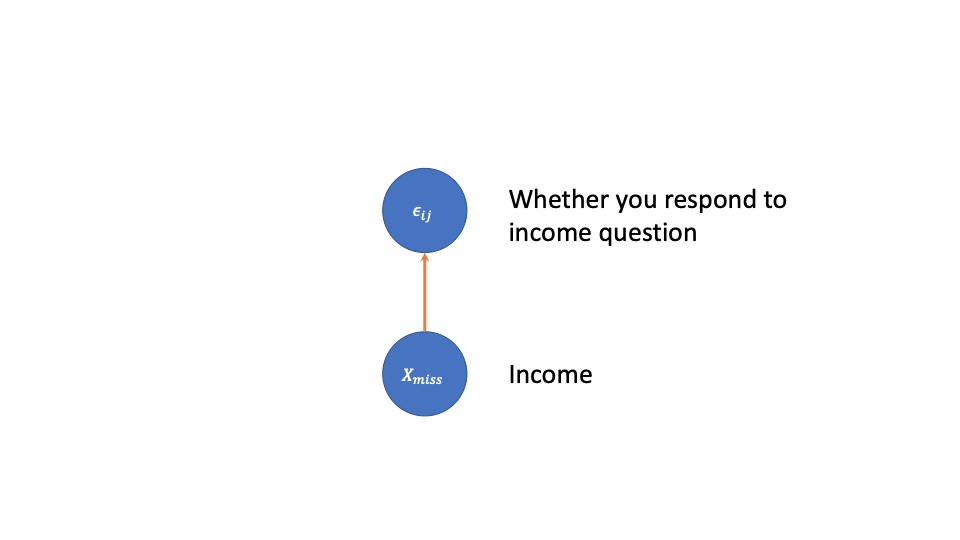
Here the missingness probability depends on the unobserved data, and possibly the observed data as well. As an example, consider the setting where if you have low income, you are more likely to decline to report it.
This setting is the most challenging to deal with.
What Does Missing Data Look Like in Major Settings
Cross-Sectional
In cross sectional data one observes multiple subjects at a single time point. For a survey setting, one might give a survey to multiple subjects once. Here one often has, for each observation, covariates and a response, and one wishes to model their relationship. The covariates could correspond to some of the survey questions, such as how much exercise you get and what you eat, and the response could correspond to a particular survey question of interest, such as how you generally feel. One observes pairs  where
where  and
and  . Examples include linear regression and standard generalized linear models (logistic regression, poisson regression, etc). Here, for each vector
  , some elements may be missing.
Time Series
This is the temporal setting for sequential data, but with only one (potentially vector-valued) sequence. Here one observes a sequence  , where each
  . Specific elements of the vector
  or the whole vector may be missing.
General examples may include returns of a stock index where some days are missing, heights of ocean spots where the instruments sometimes fail, and sales of some set of products over a  year period, where either some products or entire years are missing.
In R, the airquality dataset has missing values. This tracks ozone, solar, wind, and temperature measurements over a period from May to September. We can load and look at the data as follows
data(airquality)
head(airquality)
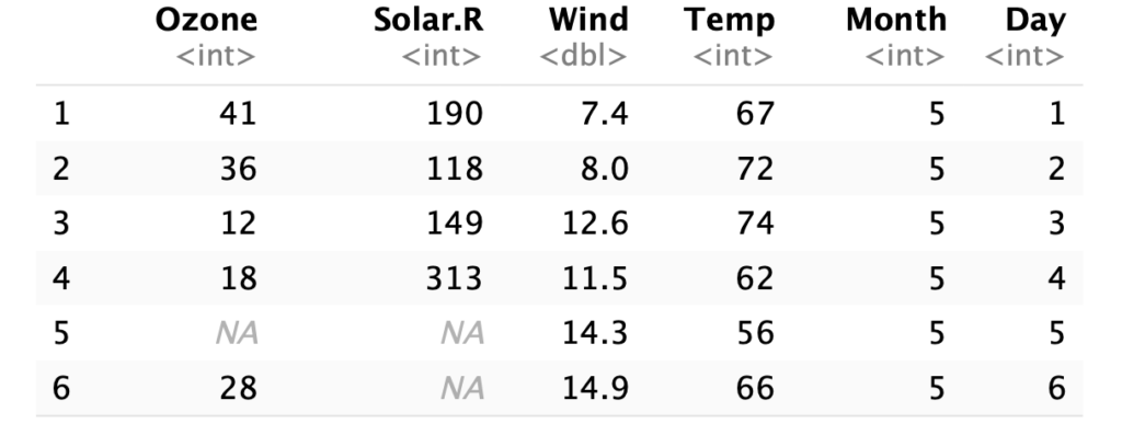
We can see that on the fifth day there are no ozone or solar measurements, and on the sixth day there were no solar measurements. Relating this back to assumptions: what would this look like:
- MCAR: the instruments failed. The missingness has no relationship to any data values.
- MAR: missingness depends on either the previous history of the variables, or on the other variables. For instance, the solar instrument might tend to fail more if wind is very high.
- MNAR: the solar instrument fails more when the sun is out, and this is not fully explained by wind or temperature.
Longitudinal
Here, we have multiple sequences, and sequences are generally considered to be independent, given their personalized characteristics of both covariates and potentially latent variables (when that assumption isn’t made the line between multivariate time series and longitudinal data becomes blurrier). For each participant , we observe  and
and  .
.
Examples could include tracking multiple patients over time and measuring biomarkers in a disease progression study. Many models for longitudinal data can handle irregularly sampled observations, such as appointment times, so it becomes important to consider assumptions relating the two.
Summary
In this post we describe the basic assumptions of missing data and what examples can look like in major settings. In future posts we will describe various ways to deal with missing data.
References
[1] Little, Roderick JA, and Donald B. Rubin. Statistical analysis with missing data. Vol. 793. John Wiley & Sons, 2019.Harvard