The Autoregressive (AR) Model

Contents hide

1 High-Level Idea

2 AR Model: Equation

3 First Steps When Fitting an AR Model

3.1 Plot and Check for Stationarity

3.2 Compare ACF and PACF

4 Fitting and Interpreting the Model

4.1 Choosing Lags

4.2 Interpreting the Model

4.2.1 Undoing the Differencing

In this post we describe the autoregressive (AR) time series model. We define it, describe steps to take before fitting one, how to choose the number of lags, and how to interpret the resulting fitted model.

High-Level Idea

The autoregressive model posits that values of a time series are correlated with and depend on recent past values. Intuitive examples may include: moods tend to persist but return to baseline and sales tend to persist. In particular, the model describes how recent past values or ‘lags’ linearly affect the current value of a time series.

AR Model: Equation

Let $y_1,\cdots, y_T$ be a univariate time series. An AR(p) model states

(1) $\begin{align*}y_t&=\beta_0+\beta_1 y_{t-1}+\cdots+\beta_p y_{t-p}+\epsilon_t\end{align*}$

here $\epsilon_t$ is a white noise process. If it is an independent white noise process then $p(y_t|y_1,\cdots,y_{t-1})=p(y_t|y_{t-p},\cdots,y_{t-1})$ i.e. we have a Markov property.

First Steps When Fitting an AR Model

Plot and Check for Stationarity

We should first visualize the time series and check for stationarity. We want both constant mean and constant autocovariance. Without stationarity the resulting model will be wrong: often either the white noise process assumption will be violated or the process will be explosive. Let’s load the BJsales dataset and plot it.

library(tseries)
data('BJsales')
plot(BJsales)

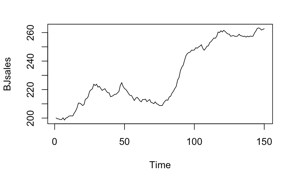
This clearly has a trend. Let’s first difference and look again.

plot(diff(BJsales))

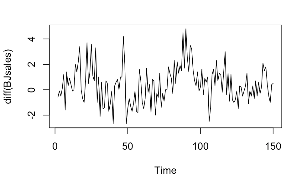
This looks somewhat better. The variance seems to be changing over time though: sometimes it looks small for a while and then we see periods with larger jumps. Let’s do an augmented Dickey Fuller test to check more formally.

print(adf.test(diff(BJsales)))

	Augmented Dickey-Fuller Test

data:  diff(BJsales)
Dickey-Fuller = -3.3485, Lag order = 5, p-value = 0.06585
alternative hypothesis: stationary

It’s on the border with a p-value of 0.066. It’s not perfect but we can use it. We could difference again but for this exercise we won’t.

Compare ACF and PACF

The next step is to compare the ACF and PACF plots. In order to decide to use an AR(p) model, we should see approximately geometric decay in the ACF plot, and p significant terms in the PACF plot.

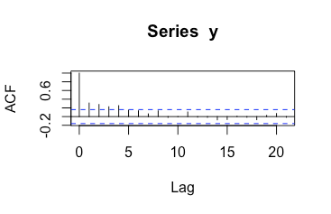
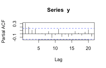
It looks like the ACF plot has approximately geometric decay, while the PACF plot has two significant terms. This suggests an AR(2) model.

Fitting and Interpreting the Model

Choosing Lags

There are two standard ways to choose lags. One is to use the PACF plot as we did above, and one is to use AIC. Based on the pacf plot we choose an AR(2) model. We also fit a model fit using AIC to choose lags.

ar_model_pacf

Call:
ar(x = y, aic = FALSE, order.max = 2)

Coefficients:
     1       2  
0.2493  0.2005  

Order selected 2  sigma^2 estimated as  1.832

ar_model_aic

Call:
ar(x = y, aic = TRUE)

Coefficients:
     1       2       3       4  
0.2123  0.1493  0.0776  0.1383  

Order selected 4  sigma^2 estimated as  1.8

Interpreting the Model

The first model, chosen using the pacf plot, tells us

(2) $\begin{align*}\hat{y}_t=0.2493y_{t-1}+0.2005y_{t-2}\end{align*}$

this says that the fitted difference between this period’s sales and last period’s sales is 0.2493 times the difference one period ago plus 0.2005 times the difference two periods ago.

Undoing the Differencing

However let’s say we want to predict the actual sales and not the changes in sales, or describe the model for actual sales. Let $z_t$ be the sales at time $t$ . Then

(3) $\begin{align*}y_t&=z_t-z_{t-1}\\z_t&=y_t+z_{t-1}\\\hat{z}_t&=0.2493(z_{t-1}-z_{t-2})+0.2005(z_{t-2}-z_{t-3})+z_{t-1}\\&=1.2493z_{t-1}-0.0488z_{t-2}-0.2005z_{t-3}\end{align*}$