Binary Classification in R: Logistic Regression, Probit Regression and More

In this post we describe how to do binary classification in R, with a focus on logistic regression. Some of the material is based on Alan Agresti’s book [1] which is an excellent resource.

For many problems, we care about the probability of a binary outcome taking one value vs. another. For instance, we might ask: what is the probability that:

someone has a disease?
some employee will quit within x months?
a customer buys something?

We’re interested both in specific predictions, and in describing how the values of features relate to these questions. For instance, how much does a unit change in a blood measurement change the disease probability? We are interested in using probabilities for classification because we’d like to characterize how certain we are in our predictions, as well as describe how much a change in a feature changes the probability of occurrence. We’d also like for features to have a bigger impact on probabilities when we’re more uncertain.

Logistic regression vs linear regression: Why shouldn’t you use linear regression for classification?

Above we described properties we’d like in a binary classification model, all of which are present in logistic regression. What if we used linear regression instead? There are several problems:

Linear regression assumes normally distributed errors for hypothesis testing
Linear regression does not output probabilities. We can somewhat characterize uncertainty by distance from the decision boundary, but it’s far less intuitive.
For classification, linear regression is very sensitive to outliers.

Let’s look more closely at the last point. Consider a ground truth model where we only have one feature $x$ :

$y=1$ if $x>0$
$y=-1$ if $x<0$

Let’s generate data from such a model in R without outliers in the features and fit a linear model.

x=c(-2,-1,1,2)
y=(x>0)
y[y==FALSE]=-1
y[y==TRUE]=1
plot(x,y)
abline(lm(y~x),col='red')

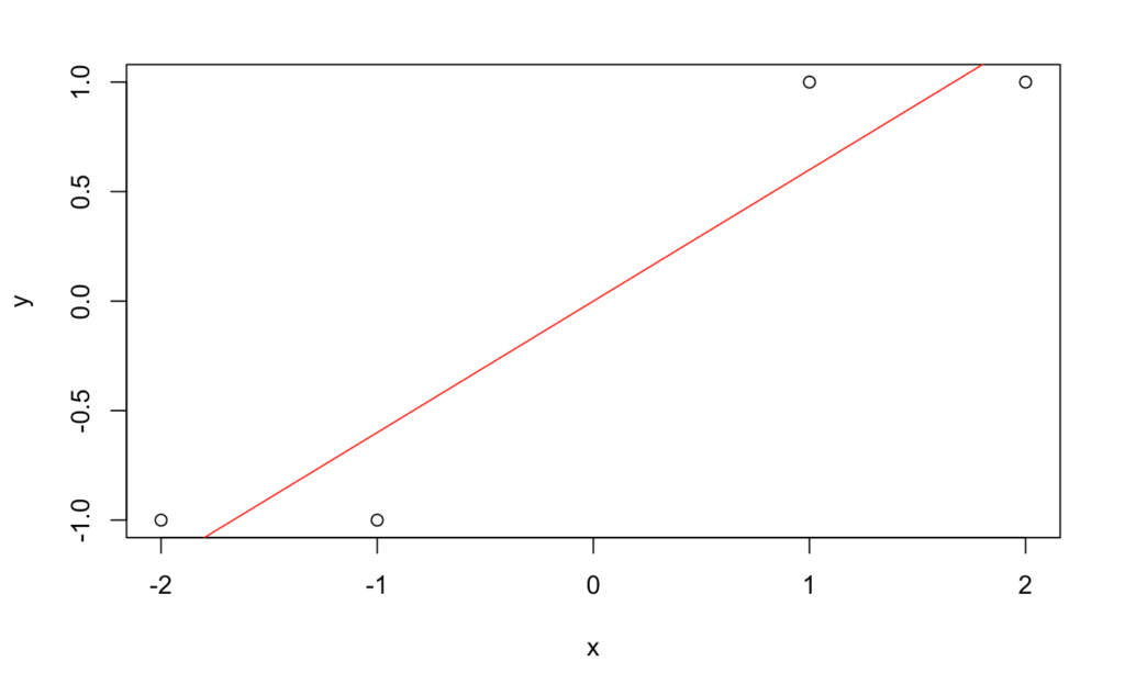
This looks reasonable. Now let’s look at the coefficients and try predicting $y$ for $x=0.25$ .

#Here we print coefficients
lm(y~x)
#Here we predict on a new value
coef(summary(lm(y~x)))[1,1]+0.25*coef(summary(lm(y~x)))[2,1]

Call:
lm(formula = y ~ x)

Coefficients:
(Intercept)            x  
        0.0          0.6  

[1] 0.15

We can assign class $1$ to any prediction greater than $0$ and $-1$ to any less than $0$ . Since we predicted $0.15$ , we predicted the correct class.

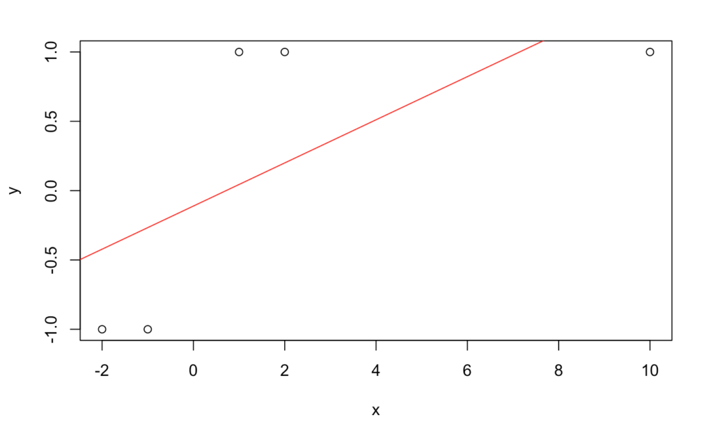
Now let’s add an outlying feature of $x=10$ and make the same plot and prediction.

x=c(-2,-1,1,2,10)
y=(x>0)
y[y==FALSE]=-1
y[y==TRUE]=1
plot(x,y)
abline(lm(y~x),col='red')
lm(y~x)
coef(summary(lm(y~x)))[1,1]+0.25*coef(summary(lm(y~x)))[2,1]

Call:
lm(formula = y ~ x)

Coefficients:
(Intercept)            x  
    -0.1111       0.1556  

[1] -0.07222222

As we can see here, the prediction is now for the wrong class simply due to adding one outlying feature with the correct label. The image shows how the slope has changed due to the new feature. Also, while we know that predictions close to $0$ are less certain, we don’t have a good way of characterizing how uncertain they are compared to a prediction of say $3$ or $-3$ .

While letting $y=1,-1$ was useful here for illustrative purposes. Going forward we use $y=1,0$ , as the math works out better.

Grouped vs Ungrouped Data

An important consideration for binary classifiers is whether one deals with grouped or ungrouped data. In grouped data, there is a fixed number of possible covariate patterns, $N$ . This occurs due to categorical features. The number of replicates in each group can be represented by a vector $\boldsymbol{n}=(n_1,n_2,\cdots,n_N)$ . Each $n_i$ represents the number of Bernoulli trials in a Binomial observation, and $n_i y_i\sim$ bin $(n_i,\pi_i)$ , where $\pi_i$ is the probability of observing a $1$ for group $i$ , i.e. under covariate pattern $i$ . That is, we assume that two observations sharing a covariate pattern imply the same distribution in the response. Note that often $\pi_i$ is termed the ‘success’ probability: however, often in classification it can refer to the probability of a bad event, so we will avoid calling it that.

In ungrouped data the covariate pattern for each observation is unique, so that we have $\boldsymbol{n}=(1,1,\cdots,1)$ repeated $N$ time, where in this case we have $N$ Bernoulli observations, each with a different probability of observing label $1$ .

Given this setup and some features for group $X^{(i)}$ , which may represent either an individual or a group, we want to use these features to predict $\pi_i$ , the probability of label $1$ , as well as do inference on the relationship between $X^{(i)}$ and $\pi_i$ .

Latent Variable Interpretation

Recall how, when describing why linear regression is problematic for classification, we defined $y$ as taking values $1$ or $-1$ based on whether $x$ was positive or negative. This is a threshold model. Many classifiers can be interpreted as threshold models. In this setting, we have an unobserved continuous response $y_i^*=\sum_j \beta_j X^{(i)}_j+\epsilon_i$ , where $\epsilon_i$ is noise, and our observed binary response $y_i$ summarizes whether $y_i^*$ is above or below a threshold $\tau$ . Then

$y_i=1$ if $y_i^*>\tau$
$y_i=0$ if $y_i^*\leq \tau$

Letting $F$ be the CDF for $\epsilon_i$ , we have

(1) $\begin{align*}P(y_i=1)&=P(y_i^*>\tau)\\&=P(\sum_j \beta_j X^{(i)}_j+\epsilon_i>\tau)\\&=1-P(\epsilon_i\leq \tau-\sum_j \beta_j X^{(i)}_j)\\&=1-F(\tau-\sum_j\beta_j X^{(i)}_j)\end{align*}$

We can set $\tau=0$ and then choose $F$ to be some distribution that is symmetric about $0$ , giving us

(2) $\begin{align*}F(z)&=1-F(-z)\\P(y_i=1)&=F(\sum_j\beta_j X^{(i)}_j)\\F^{-1}(P(y_i=1))&=\sum_j\beta_j X^{(i)}_j\end{align*}$

If we let $y_i$ take values $1$ and $0$ only, then we have $P(y_i=1)=E(y_i)$ . Thus

(3) $\begin{align*}F^{-1}(E(y_i))&=\sum_j\beta_j X^{(i)}_j\end{align*}$

which tells us that we can use the inverse CDF from this latent variable representation as the link function in a generalized linear model. Two common choices for $F$ are the logistic distribution and the standard normal distribution. The first leads to logistic regression, and the second to probit regression. The logistic distribution CDF is

(4) $\begin{align*}F(z)&=\frac{\exp(z)}{1+\exp(z)}\end{align*}$

which leads to the following forms for the probability of observing a $1$ $\pi_i$ ,

(5) $\begin{align*}\pi_i&=\frac{\exp(\sum_j\beta_j X^{(i)}_j)}{1+\exp(\sum_j\beta_j X^{(i)}_j)}\\\textrm{logit}(\pi_i)&=\log \frac{\pi_i}{1-\pi_i}\\&=\sum_j \beta_j X^{(i)}_j\end{align*}$

here $\frac{\pi_i}{1-\pi_i}$ is called the odds ratio or the odds. We will discuss the interpretation of this in more detail when we look at example data.

GLM Interpretation

All of the above leads up to a generalized linear model (GLM) formulation. A GLM has three parts:

a linear predictor
an exponential family distribution
a link function

Our linear predictor is clear. Our exponential is binomial $n_i,\pi_i$ for each group, and our link function is the inverse of the logistic CDF, which is the logit function.

Fitting Logistic Regression in R

Let’s load the Pima Indians Diabetes Dataset [2], fit a logistic regression model naively (without checking assumptions or doing feature transformations), and look at what it’s saying.

diabetes<-read.csv(url('https://raw.githubusercontent.com/jbrownlee/Datasets/master/pima-indians-diabetes.data.csv'))
head(diabetes)

   X6 X148 X72 X35  X0 X33.6 X0.627 X50 X1
1  1   85  66  29   0  26.6  0.351  31  0
2  8  183  64   0   0  23.3  0.672  32  1
3  1   89  66  23  94  28.1  0.167  21  0
4  0  137  40  35 168  43.1  2.288  33  1
5  5  116  74   0   0  25.6  0.201  30  0
6  3   78  50  32  88  31.0  0.248  26  1

The column descriptions are as follows:

X6: # of times pregnant
X148: plasma glucose concentration
X72: blood pressure
X35: skin thickness
X33.6: insulin
X0.627: diabetes pedigree function
X50: age
X1: 1 if diabetes, 0 otherwise

We can then fit a logistic regression model and look at the output

classifier <- glm(X1~X6+X148+X72+X35+X0+X33.6+X0.627+X50,family='binomial',data=diabetes)
classifier

Call:  glm(formula = X1 ~ X6 + X148 + X72 + X35 + X0 + X33.6 + X0.627 + 
    X50, family = "binomial", data = diabetes)

Coefficients:
(Intercept)           X6         X148          X72          X35           X0        X33.6  
 -8.3862464    0.1232043    0.0350533   -0.0132215    0.0003301   -0.0011554    0.0897505  
     X0.627          X50  
  0.9414265    0.0146080  

Degrees of Freedom: 766 Total (i.e. Null);  758 Residual
Null Deviance:	    991.4 
Residual Deviance: 722.8 	AIC: 740.8

Interpreting Logistic Regression Coefficients

We now have the coefficients, and would like to interpret them. In the linear regression, the coefficients tell us about the expected change in the response due to a unit change in the feature. Here, we only know directly about the change in the linear predictor, although we can still say something about the response.

There are two primary ways to use the coefficient to tell us about the response: looking at the rate of change or partial derivative of the probability of a $1$ $\pi_i$ with respect to a feature, or looking at how the odds change with a unit change in the feature.

For the first, the partial derivatives are given by

(6) $\begin{align*}\frac{\delta\pi_i}\frac{\delta X^{(i)}_j}&=\beta_j\frac{\exp(\sum_k \beta_k X^{(i)}_k)}{1+\exp(\sum_k \beta_k X^{(i)}_k}\\&=\beta_j \pi_i(1-\pi_i)\end{align*}$

this tells us that changes close to $\pi_i=0.5$ , i.e. close to the decision boundary, have a smaller effect than changes further from it. However, it is a bit unwieldy to use as we need to fix the feature values, so we won’t use it here.

The more useful interpretation comes from the odds ratio $\pi_i/(1-\pi_i)$ . We can calculate the multiplicative effect of a feature on the odds ratio via

exp(coef(classifier))

(Intercept)           X6         X148          X72          X35           X0        X33.6 
0.0002279814 1.1311154752 1.0356749491 0.9868654931 1.0003301125 0.9988453120 1.0939013662 
      X0.627          X50 
2.5636359321 1.0147152119

This tells us, for each feature, how much a unit change in the feature changes the odds ratio multiplicatively. The odds tell us how much more ‘likely’ an outcome of $1$ is than an outcome of $0$ .

Here, a unit change in # of times pregnant increases the odds of diabetes by a factor 1.13, while a unit change in diabetes pedigree function increases the odds by a factor of 2.56.

Conclusion

In this post, we described binary classification with a focus on logistic regression. We described why linear regression is problematic for binary classification, how we handle grouped vs ungrouped data, the latent variable interpretation, fitting logistic regression in R, and interpreting the coefficients. In the future we may discuss the details of fitting, model evaluation, and hypothesis testing.

[1] Agresti, Alan. Foundations of linear and generalized linear models. John Wiley & Sons, 2015.
[2] Dua, D. and Graff, C. (2019). UCI Machine Learning Repository [http://archive.ics.uci.edu/ml]. Irvine, CA: University of California, School of Information and Computer Science.