In this post we show how to predict future measurement values in a longitudinal setting using linear mixed models (LMMs). We describe how to do it in R, and how to evaluate the accuracy, which requires somewhat careful handling.
The Problem and Dataset
In a previous post we went over the more methodological side of LMMs. However, we did not show how to do prediction of future values or evaluate those predictions. We will work with the aids dataset from the joineR package. This is a dataset of CD4 (white blood cell) count measurements along with death or censoring times as well as some covariates/treatment indicators. We will ignore the death/censoring times and focus on CD4 count measurement times (technically we should do a joint model, as the death/event times tell us something about what the unseen CD4 counts are close to those times, and thus the CD4 dynamics, but we will ignore death/censoring times for simplicity).
We start by loading packages and the dataset.
library(joineR)
library(lme4)
library(splines)
library(caret)#we will use this for cross validation
library(scorer)#we will use this to calculate mean absolute and squared error

data(aids)
head(aids)
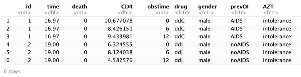
The columns give the following information:
- id: the id of the patient
- time: the death or censoring time
- death: whether the patient died while observed
- CD4: the CD4 count
- obstime: how many months from the first observation this is
- drug: the treatment type
- gender: male or female
- prevOi: whether there was a previous infection
- AZT: AZT intolerance or failure
Independence and Evaluation Metrics
We will want to construct confidence intervals for our accuracy metrics. To do so, we need to think about independence. We should first note that our within subjects measurements are not iid. We can assume that patients are all realizations of the same stochastic process and independent of each other though. However, CD4 measurements within a patient may depend on each other. Thus, we should average our accuracy metrics within subject, and use within-subject averages to construct confidence intervals and other relevant summary statistics. To start with, we perform k-fold cross validation and create k folds, as well as set up data structures to hold our within-subject mean absolute errors (MAEs) and mean squared errors (MSEs) for each patient, for both linear regression (LM) and a linear mixed model (LMM).
all_participants<-unique(aids[['id']])
#we create cross validation folds using caret's createFolds
num_folds <- 10
folds<-createFolds(all_participants,k=num_folds,list=TRUE,returnTrain=TRUE)
#data structures to hold results
MAE_within_subjects_lm <- c()
MAE_within_subjects_lmm <- c()
MSE_within_subjects_lm <- c()
MSE_within_subjects_lmm <- c()
Next, for each fold, we train our model and make predictions. We will use all covariates along with a random intercept for the mixed model. We then save the our within-subjects MAEs and MSEs in the relevant data structures.
The Experiment
for(i in 1:num_folds){
  train_ids<- folds[[i]]
  test_ids<-all_participants[!(all_participants%in%folds[[i]])]
  #generate train/test
  train<-subset(aids,id%in%train_ids)
  test<-subset(aids,id%in%test_ids)
  #fit models
  aids_lm <- lm(formula=CD4~obstime+drug+gender+prevOI+AZT,data=train)
  aids_lmm <-lmer(formula=CD4~obstime+drug+gender+prevOI+AZT+(1|id),data=train)
  test_participants <- unique(test[['id']])
  for(participant in test_participants){
    prediction_subset <- subset(test,id==participant)
    #predict
    y_pred_lm <- predict(aids_lm,newdata=prediction_subset)
    y_pred_lmm <- predict(aids_lmm,newdata=prediction_subset,allow.new.levels=TRUE)
    y_true <- prediction_subset[['CD4']]
    MAE_within_subjects_lm<- c(MAE_within_subjects_lm,mean_absolute_error(y_pred_lm,y_true))
    MAE_within_subjects_lmm<- c(MAE_within_subjects_lmm,mean_absolute_error(y_pred_lmm,y_true))
    MSE_within_subjects_lm<-c(MSE_within_subjects_lm,mean_squared_error(y_pred_lm,y_true))
    MSE_within_subjects_lmm<-c(MSE_within_subjects_lmm,mean_squared_error(y_pred_lmm,y_true))
  }
}
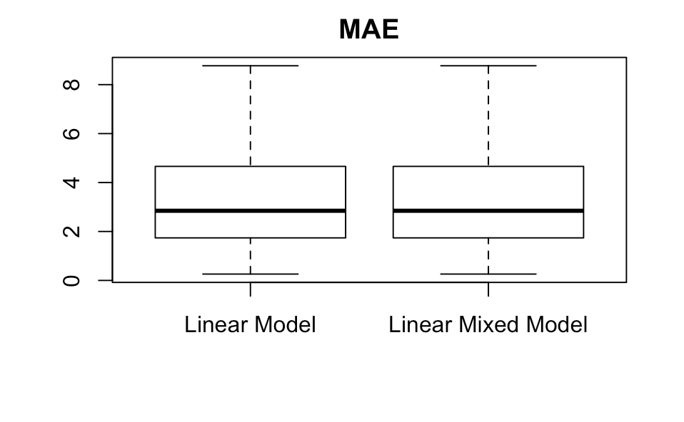
Using these, we can make boxplots. We remove the outliers to improve clarity.
boxplot(MAE_within_subjects_lm,MAE_within_subjects_lm,main='MAE',names=c('Linear Model','Linear Mixed Model'),outline=FALSE)
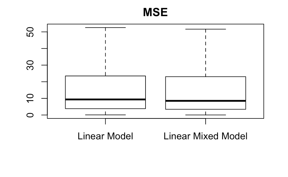
boxplot(MSE_within_subjects_lm,MSE_within_subjects_lmm,main='MSE',names=c('Linear Model','Linear Mixed Model'),outline=FALSE)
Let’s look at  confidence intervals for the mean.
t.test(MAE_within_subjects_lm)
t.test(MAE_within_subjects_lmm)
t.test(MSE_within_subjects_lm)
t.test(MSE_within_subjects_lmm)
| MAE | MSE | |
| LM | (3.250611, 3.681545) | (16.78123, 21.41477) |
| LMM | (3.197386, 3.642805) | (16.71764, 21.56956) |
The linear mixed model performs better than the linear model on these two metrics, but just barely, and even without showing the two-sample hypothesis test we can tell that the difference is not significant. Why might this be?
Why Doesn’t the Linear Mixed Model do Better
Here are a few obvious reasons: we will focus on the first three
- The covariates explain most of the patient specific variation
- There is a lot of noise
- something is wrong with our model specification for patient specific variation
We would like to test the first one. Let  be the variance of the random intercept. Then


Note that  is on the boundary of the parameter space, which makes testing problematic. However, we can still look at the variance even if we don’t make a formal test. Let’s fit the mixed model on the whole dataset and investigate this.
aids_mixed_all <-lmer(formula=CD4~obstime+drug+gender+prevOI+AZT+(1|id),data=aids)
summary(aids_mixed_all)
I’ll extract the relevant part of this summary:
Random effects:
 Groups   Name        Variance Std.Dev.
 id       (Intercept) 15.253   3.905
 Residual              3.842   1.960
Number of obs: 1405, groups:  id, 467
This variance is pretty large and seems unlikely to be due to chance. Now for the second issue (lots of noise), I don’t know of a formal hypothesis test, but we can look at both the residual standard error and the  for the linear regression model with fixed effects only. That said, there are a lot of reasons why will be low or residual standard error will be high, many of which relate to various types of model misspecification rather than noise.
aids_lm_all <- lm(formula=CD4~obstime+drug+gender+prevOI+AZT,data=aids)
summary(aids_lm_all)

Call:
lm(formula = CD4 ~ obstime + drug + gender + prevOI + AZT, data = aids)

Residuals:
     Min       1Q   Median       3Q      Max
-10.5414  -3.0200  -0.8382   2.5663  16.0378

Coefficients:
            Estimate Std. Error t value Pr(>|t|)
(Intercept) 10.53580    0.45676  23.066  < 2e-16 ***
obstime     -0.08396    0.02525  -3.325 0.000905 ***
drugddI      0.50938    0.23679   2.151 0.031628 *
gendermale  -0.68624    0.43070  -1.593 0.111314
prevOIAIDS  -4.43438    0.29602 -14.980  < 2e-16 ***
AZTfailure  -0.15939    0.30194  -0.528 0.597656
---
Signif. codes:  0 ‘***’ 0.001 ‘**’ 0.01 ‘*’ 0.05 ‘.’ 0.1 ‘ ’ 1

Residual standard error: 4.433 on 1399 degrees of freedom
 Multiple R-squared:  0.2036,    Adjusted R-squared:  0.2007
We see that the is low. To evaluate the residual standard error, let’s look at the box plot for the CD4 values. Note that there is a problem here: CD4 values are likely not independent from each other, so this box plot will probably underestimate the quantiles distance from the median. However, it’s still somewhat interesting.
boxplot(aids[['CD4']],main='CD4 value box plot')
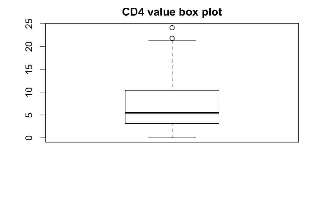
We can see that the lower quantile is close to  and the upper quantile is close to
  , so our residual standard error of
  is quite large, even if the true quantiles are probably more spread out.
In conclusion, in this post, we showed how to do prediction with k-fold cross validation using linear mixed models. We constructed box plots and made confidence intervals for the mean for both within-subjects MAE and within-subjects MSE. We also investigated why the linear mixed model didn’t do much better than the fixed effects only linear model.
Hi there,
I am trying to adapt this code to assess the accuracy of a logistic mixed model. I am trying to assess whether this code is useful to run a confusion matrix, but I am not sure that’s it’s actually doing what I hope it’s doing and I having trouble understanding what the code is doing in line with notes after the ## below. I have a few more questions, but I thought I would keep it simple in case elicits a faster response, but if there is someone who could clarify further, that would be greatly appreciated. Thanks so much for your time.
for(i in 1:num_folds){
train_ids<- folds[[i]]
test_ids<-all_participants[!(all_participants%in%folds[[i]])] ## is this leaving out one participant? Or testing for EACH participant?
#generate train/test
train<-subset(aids,id%in%train_ids)
test<-subset(aids,id%in%test_ids)
#fit models
aids_lm <- lm(formula=CD4~obstime+drug+gender+prevOI+AZT,data=train)
aids_lmm <-lmer(formula=CD4~obstime+drug+gender+prevOI+AZT+(1|id),data=train)
test_participants <- unique(test[['id']])
for(participant in test_participants){
prediction_subset <- subset(test,id==participant)
#predict
y_pred_lm <- predict(aids_lm,newdata=prediction_subset)
y_pred_lmm <- predict(aids_lmm,newdata=prediction_subset,allow.new.levels=TRUE)
y_true <- prediction_subset[['CD4']]
MAE_within_subjects_lm<- c(MAE_within_subjects_lm,mean_absolute_error(y_pred_lm,y_true))
MAE_within_subjects_lmm<- c(MAE_within_subjects_lmm,mean_absolute_error(y_pred_lmm,y_true))
MSE_within_subjects_lm<-c(MSE_within_subjects_lm,mean_squared_error(y_pred_lm,y_true))
MSE_within_subjects_lmm<-c(MSE_within_subjects_lmm,mean_squared_error(y_pred_lmm,y_true))
}
}
Hi Cassie,
That part holds out all the participants who are not in the current fold to create the test set, trains on everyone else, and then predicts on the test set.
Best,
Alex