In this post we describe the basics of long-short term memory (LSTM). We first describe some alternative classical approaches and why they are unsatisfactory for the types of problems LSTM handles, then describe the original recurrent neural (RNN) and its limitations, and finally describe LSTM.
In many settings, we want to do time series classification of a response using both current features/inputs and historical information about both previous features and potentially previous responses. For instance, in the MIMIC-III dataset [1], we may want to predict whether a patient will experience a same-day or next-day sepsis using features such as their vital signs, lab results, demographic data, and prescribed medication.
Note that technically prescribed medication is quite different as it is a treatment while vital signs, lab results, and demographic data are (potentially time-varying) covariates. However, for this setting we will ignore this issue and treat medication as a covariate.
Classical Models: Non-Temporal Classification
The simplest way to do this is with a non-temporal classifier. We could use logistic regression, Naive Bayes, SVM, or a deep neural network. However, this has the problem that dependency on the past may matter. For instance, say someone has received a drug: how long ago one received it may matter. Similarly, while you are primarily interested in whether someone will develop Sepsis, whether someone has it or not also will likely be predictive of whether they will continue to not have it/have it. Temporal models provide a way to handle this.
Classical Models: Autoregressive Models, AR(1), etc.
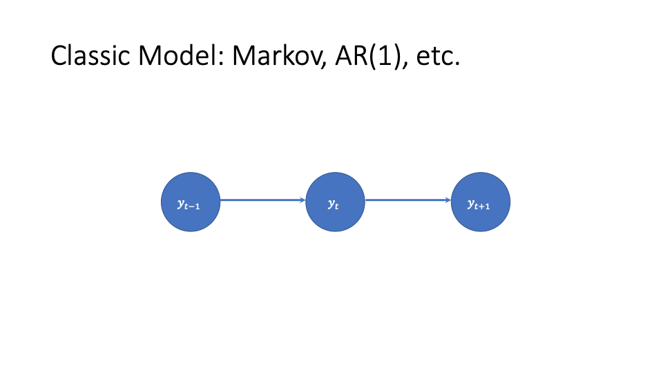
A simple temporal model for the response has it depend only on its previous value: this is a first order Markov process. A special case of this is an autoregressive order-1 process with independent errors. In equations this is
(1) 
For a generalized linear model like logistic regression we might have.
(2) 
One can extend to multiple previous values via an AR(k) or k-th order Markov model. For the MIMIC-III case, this model incorporates the previous history of Sepsis, but not the time-varying covariates like vital signs. We need some way to incorporate them.
Adding Time-Varying Covariates
We can add time-varying covariates as follows.
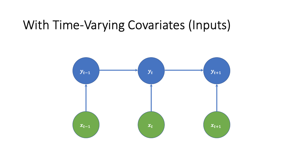
In the GLM case, this would look like
(3) 
however, we’d like a few things that this model has difficulty with:
- handle flexible non-linearity
- have longer term dependence on past covariates and/or responses. In particular, this structure causes the effect of drugs that are not baseline covariates to disappear the next day. If you want to fix that, you need to add connections between covariates and future responses, and choose those connections by hand. Depending on your structure this may make learning more challenging.
- in line with the previous, we want to have less feature selection.
Recurrent Neural Networks
One way to handle this is to add a hidden state. This can give us non-linearity, it allows dependence on the past without explicitly specifying how many time steps to keep it for via the graphical model structure, and it lets us avoid handcrafting features.
We then have the following architecture
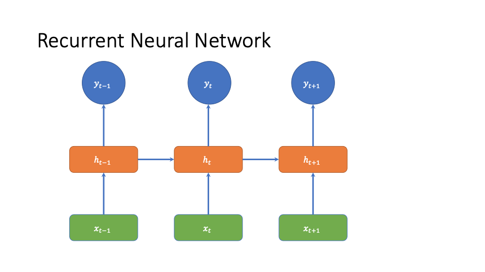
This architecture solves many of the issues described above. Thanks to the hidden layer, we don’t have to directly link previous medications to future time steps, we can do at least some feature learning automatically, and we get flexible non-linearity.
However, this has the problem that the effect of old information decays exponentially over time (see https://www.cs.toronto.edu/~graves/phd.pdf figure 4.1). This leads to the well known vanishing gradient problem in training (also https://www.cs.toronto.edu/~graves/phd.pdf figure 4.1), but also leads to issues with a learned model. In particular, some medications will have different effect decay rates with different functional forms. The exponential decay cannot capture that.
LSTM
To handle this, LSTM proposes using gates and cells: I’m going to describe them in a slightly non-standard way that I find clearer, while referencing the way that they’re described in Wikipedia. Intuitively, the cell describes the information that goes into the hidden layer, and the gates weight information that eventually goes into the hidden layer, at different stages. Now I’ll directly copy some text and equations from the wikipedia page, and then describe their intuition in more detail.
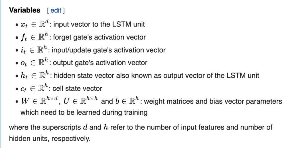
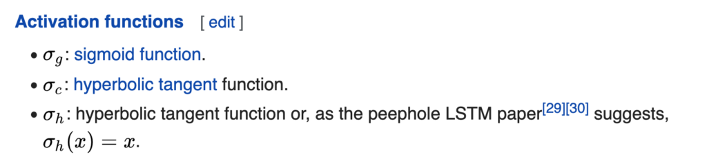
Wikipedia Equations
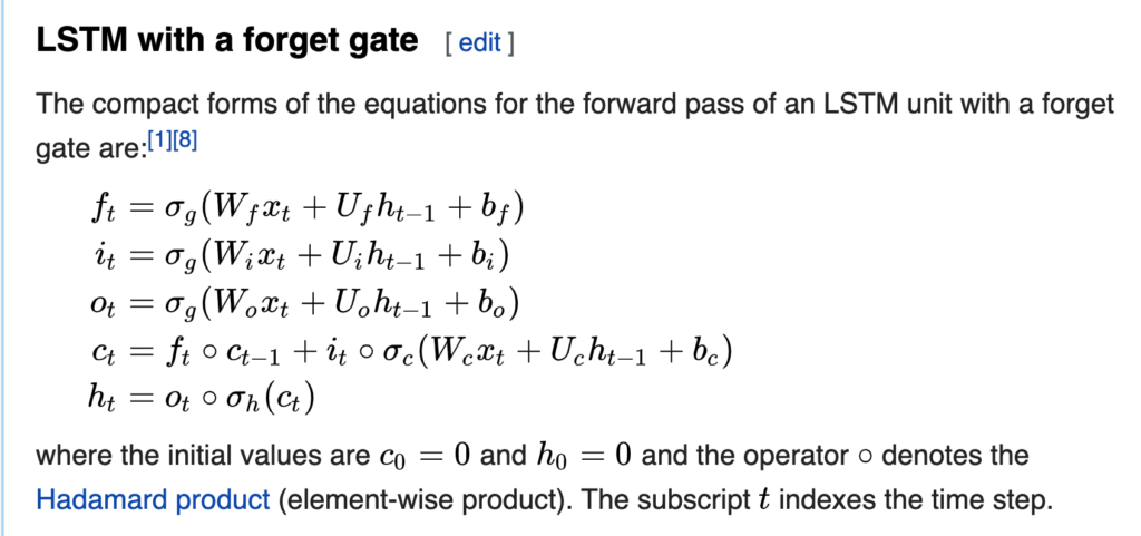
High-Level Ideas
We have three gates: the forget, input, and output gate. Each applies the same activation function to affine transformations of the same features (the previous hidden state), but if you look at how they’re used, they’re used to weight information at various stages. The forget gate weights the previous cell state: you can think of this as how much extra weight do we give to old information beyond a ‘regular’ RNN? The input gate weights  , which is the same functional form you might see for the hidden layer you would see in a regular RNN. One way to think about it is: how much weight do we give the ‘regular’ RNN part. Finally, the output gate weights the components of the output of an activation function applied to the cell.
The cell itself is often described as the memory. We can think of this as a vector-weighted sum of previous information that went into the previous hidden state, and terms that would determine the hidden state of a ‘regular’ RNN.
Gates for the Sepsis Problem
So how would you interpret each of these in terms of medicines and labs?
- forget gate: based on current labs/medications and the previous summary (hidden state), how much extra weight do we give to the past labs/medications?
- input gate: how much weight do we assign to a model that assumes exponential decay of the importance previous medicines and lab readings?
- cell gate: our weighted summary of both the exponential decay model and the extra weight given to past labs/medications, where weights are determined by the forget gate and input gate. This gives us the main information that will eventually go into the hidden state.
- output gate: using current labs/medications to weight an activation function applied to the cell gate.
Conclusion
In conclusion, often we want to do time series classification for some problem. When we would like flexible non-linearity, feature learning, and to not directly specify the number of time steps of dependence the present has on the past, we can use RNNs. However, to have more flexibility in the decay rate of old information, we can use LSTMs.
[1] MIMIC-III, a freely accessible critical care database. Johnson AEW, Pollard TJ, Shen L, Lehman L, Feng M, Ghassemi M, Moody B, Szolovits P, Celi LA, and Mark RG. Scientific Data (2016). DOI: 10.1038/sdata.2016.35. Available at: http://www.nature.com/articles/sdata201635
[2] Hochreiter, Sepp, and Jürgen Schmidhuber. “Long short-term memory.” Neural computation 9, no. 8 (1997): 1735-1780.