Linear Regression Summary(lm): Interpretting in R

Contents hide

1 Introduction to Linear Regression Summary Printouts

2 Residual Summary Statistics

4 Assessing Fit and Overall Significance

4.1 Residual Standard Error

4.2 Multiple and Adjusted

4.3 F-Statistic and F-test

Introduction to Linear Regression Summary Printouts

In this post we describe how to interpret the summary of a linear regression model in R given by summary(lm). We discuss interpretation of the residual quantiles and summary statistics, the standard errors and t statistics , along with the p-values of the latter, the residual standard error, and the F-test. Let’s first load the Boston housing dataset and fit a naive model. We won’t worry about assumptions, which are described in other posts.

library(mlbench)
data(BostonHousing)
model<-lm(log(medv) ~ crim + rm + tax + lstat , data = BostonHousing)
summary(model)

Call:
lm(formula = log(medv) ~ crim + rm + tax + lstat, data = BostonHousing)

Residuals:
     Min       1Q   Median       3Q      Max 
-0.72730 -0.13031 -0.01628  0.11215  0.92987 

Coefficients:
              Estimate Std. Error t value Pr(>|t|)    
(Intercept)  2.646e+00  1.256e-01  21.056  < 2e-16 ***
crim        -8.432e-03  1.406e-03  -5.998 3.82e-09 ***
rm           1.428e-01  1.738e-02   8.219 1.77e-15 ***
tax         -2.562e-04  7.599e-05  -3.372 0.000804 ***
lstat       -2.954e-02  1.987e-03 -14.867  < 2e-16 ***
---
Signif. codes:  
0 ‘***’ 0.001 ‘**’ 0.01 ‘*’ 0.05 ‘.’ 0.1 ‘ ’ 1

Residual standard error: 0.2158 on 501 degrees of freedom
Multiple R-squared:  0.7236,	Adjusted R-squared:  0.7214 
F-statistic: 327.9 on 4 and 501 DF,  p-value: < 2.2e-16

Residual Summary Statistics

The first info printed by the linear regression summary after the formula is the residual summary statistics. One of the assumptions for hypothesis testing is that the errors follow a Gaussian distribution. As a consequence the residuals should as well. The residual summary statistics give information about the symmetry of the residual distribution. The median should be close to $0$ as the mean of the residuals is $0$ , and symmetric distributions have median=mean. Further, the 3Q and 1Q should be close to each other in magnitude. They would be equal under a symmetric $0$ mean distribution. The max and min should also have similar magnitude. However, in this case, not holding may indicate an outlier rather than a symmetry violation.

We can investigate this further with a boxplot of the residuals.

boxplot(model[['residuals']],main='Boxplot: Residuals',ylab='residual value')

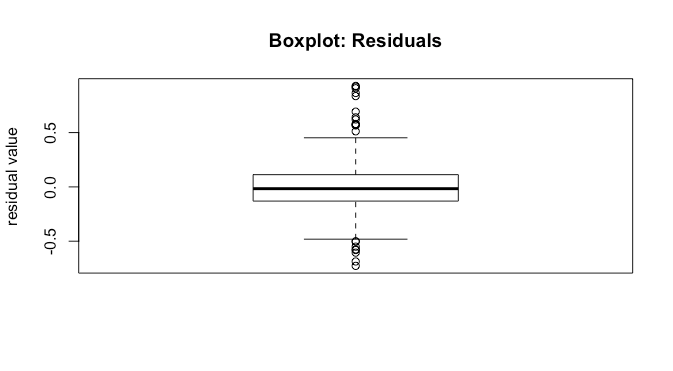
We see that the median is close to $0$ . Further, the $25$ and $75$ percentile look approximately the same distance from $0$ , and the non-outlier min and max also look about the same distance from $0$ . All of this is good as it suggests correct model specification.

Coefficients

The second thing printed by the linear regression summary call is information about the coefficients. This includes their estimates, standard errors, t statistics, and p-values.

Estimates

The intercept tells us that when all the features are at $0$ , the expected response is the intercept. Note that for an arguably better interpretation, you should consider centering your features. This changes the interpretation. Now, when features are at their mean values, the expected response is the intercept. For the other features, the estimates give us the expected change in the response due to a unit change in the feature.

Standard Error

The standard error is the standard error of our estimate, which allows us to construct marginal confidence intervals for the estimate of that particular feature. If $s.e.(\hat{\beta}_i)$ is the standard error and $\hat{\beta}_i$ is the estimated coefficient for feature $i$ , then a 95% confidence interval is given by $\hat{\beta}_i\pm 1.96\cdot s.e.(\hat{\beta}_i)$ . Note that this requires two things for this confidence interval to be valid:

your model assumptions hold
you have enough data/samples to invoke the central limit theorem, as you need $\hat{\beta}_i$ to be approximately Gaussian.

That is, assuming all model assumptions are satisfied, we can say that with 95% confidence (which is not probability) the true parameter $\beta_i$ lies in $[\hat{\beta}_i-1.96\cdot s.e.(\hat{\beta}_i),\hat{\beta}_i+1.96\cdot s.e.(\hat{\beta}_i)]$ . Based on this, we can construct confidence intervals

confint(model)
                    2.5 %        97.5 %
(Intercept)  2.3987332457  2.8924423620
crim        -0.0111943622 -0.0056703707
rm           0.1086963289  0.1769912871
tax         -0.0004055169 -0.0001069386
lstat       -0.0334396331 -0.0256328293

Here we can see that the entire confidence interval for number of rooms has a large effect size relative to the other covariates.

t-value

The t-statistic is

(1) $\begin{align*}\frac{\hat{\beta}_i}{s.e.(\hat{\beta}_i)}\end{align*}$

which tells us about how far our estimated parameter is from a hypothesized $0$ value, scaled by the standard deviation of the estimate. Assuming that $\hat{\beta}_i$ is Gaussian, under the null hypothesis that $\beta_i=0$ , this will be t distributed with $n-p-1$ degrees of freedom, where $n$ is the number of observations and $p$ is the number of parameters we need to estimate.

Pr(>|t|)

This is the p-value for the individual coefficient. Under the t distribution with $n-p-1$ degrees of freedom, this tells us the probability of observing a value at least as extreme as our $\hat{\beta}_i$ . If this probability is sufficiently low, we can reject the null hypothesis that this coefficient is $0$ . However, note that when we care about looking at all of the coefficients, we are actually doing multiple hypothesis tests, and need to correct for that. In this case we are making five hypothesis tests, one for each feature and one for the coefficient. Instead of using the standard p-value of $0.05$ , we can use the Bonferroni correction and divide by the number of hypothesis tests, and thus set our p-value threshold to $0.01$ .

Assessing Fit and Overall Significance

The linear regression summary printout then gives the residual standard error, the $R^2$ , and the $F$ statistic and test. These tell us about how good a fit the model is and whether any of the coefficients are significant.

Residual Standard Error

The residual standard error is given by $\hat{\sigma}=\sqrt{\frac{\sum \hat{\epsilon}_i^2}{n-p}}$ . It gives the standard deviation of the residuals, and tells us about how large the prediction error is in-sample or on the training data. We’d like this to be significantly different from the variability in the marginal response distribution, otherwise it’s not clear that the model explains much.

Multiple and Adjusted $R^2$

Intuitively $R^2$ tells us what proportion of the variance is explained by our model, and is given by

(2) $\begin{align*}R^2&=1-\frac{SS_{res}}{SS_{tot}}\\&=1-\frac{\sum_i\hat{\epsilon}_i^2}{\sum_i(y_i-\bar{y})^2}\end{align*}$

both $R^2$ and the residual standard standard deviation tells us about how well our model fits the data. The adjusted $R^2$ deals with an increase in $R^2$ spuriously due to adding features, essentially fitting noise in the data. It is given by

(3) $\begin{align*}\bar{R}^2&=1-(1-R^2)\frac{n-1}{n-p-1}\end{align*}$

thus as the number of features $p$ increases, the required $R^2$ needed will increase as well to maintain the same adjusted $R^2$ .

F-Statistic and F-test

In addition to looking at whether individual features have a significant effect, we may also wonder whether at least one feature has a significant effect. That is, we would like to test the null hypothesis

(4) $\begin{align*}H_0: \beta_1=\beta_2=\cdots=\beta_{p-1}=0\end{align*}$

that all coefficients are $0$ against the alternative hypothesis

(5) $\begin{align*}H_1:\exists i:1\leq i\leq p-1:\beta_i\neq 0\end{align*}$

Under the null hypothesis the F statistic will be F distributed with $(p-1,n-p)$ degrees of freedom. The probability of our observed data under the null hypothesis is then the p-value. If we use the F-test alone without looking at the t-tests, then we do not need a Bonferroni correction, while if we do look at the t-tests, we need one.