In survival analysis, we want to model the time to a first event, often death. One way to model the risk is using Cox regression, which we describe in this post. We then show a simple example.

We describe the instantaneous risk of an event via a function called the hazard. We would like to describe how this risk changes over time. We’re interested in risk changes at a global level across patients, and at an individual level in terms of covariates. Covariates can be weight, age at the start of the study, what treatment they receive, etc. Cox regression [1], a technique for describing this, specifies a global baseline hazard, which is non-parametric and thus allows the global risk to vary in a very flexible way as a function of time, and a relative risk that describes how covariates influence risk and is parametric. However, this semi-parametric specification makes inference difficult: in this article we describe this model and David Cox’s insight for how to do inference in it.

Basics of Survival Analysis

In survival analysis we want to model the probability of survival until at least time $t$ . Let $T$ be the death time. Then we want to model

(1) $\begin{align*}S(t)&=P(T>t)\\&=1-F(t)\end{align*}$

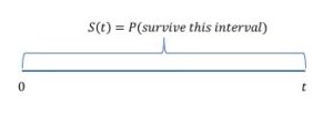
where $F(t)$ is the cumulative distribution function of the death time $T$ . The hazard is an important concept here. It is the instantaneous risk of death at time $t$ , conditional on surviving up to $t$ . For a heuristic derivation, let the conditional probability of death in the small interval $[t,t+dt)$ be given by $\lambda(t)dt$ . By rearranging terms and taking limits we obtain

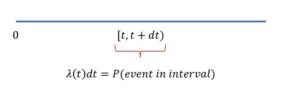
(2) $\begin{align*}\lambda(t)&=\lim_{dt\rightarrow 0}\frac{P(t\leq T\leq t+dt|T\geq t)}{dt}\end{align*}$

with some manipulation we can relate these two for continuous distributions via

(3) $\begin{align*}S(t)&=\exp(-\int_0^t \lambda(s)ds)\end{align*}$

The Cox Hazard and its Likelihood

In order to compute this, we need to specify a functional form for the hazard. Cox proposed that for an individual $n$ ,

(4) $\begin{align*}\lambda_n(t)&=\underbrace{\lambda_0(t)}_{\textrm{baseline}}\underbrace{\exp(\beta^T z_n)}_{\textrm{relative risk}}\end{align*}$

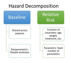
where $\lambda_0(t)$ , the baseline risk, is often taken to be non-parametric and $z_n$ is a vector of covariates for the individual $n$ . As mentioned in the introduction, the non-parametric baseline risk allows the global risk shared across patients to vary in a very flexible way, while the parametric relative risk allows us to incorporate individual covariates. However, this specification prevents us from doing maximum likelihood estimation directly. To see why, let $\delta_n$ be $1$ if the patient has their death observed and $0$ otherwise (for an example of the latter, if they survive until the end of the study or drop out). Then letting $f_n(t)$ be the density for participant $n$ and $S_n(t)$ be their survival function, the likelihood is the product of the densities for observed death times and the survival probabilities for censored patients. This gives

(5) $\begin{align*}\prod_{n=1}^N f_n(t)^{\delta_n}S_n(t)^{1-\delta_n}&=\prod_{n=1}^N (-S_n'(t))^{\delta_n} S_n(t)^{1-\delta_n}\\&=\prod_{n=1}^N [(\lambda_n(t) S_n(t)]^{\delta_n} S_n(t)^{1-\delta_n}\\&=\prod_{n=1}^N [\lambda_0(t)\exp(\beta^T z_n)]^{\delta_n} S_n(t)\end{align*}$

The Partial Likelihood

Note that in the previous likelihood, we have the nuisance parameter $\lambda_0(t)$ , which is non-parametric. We thus cannot directly maximize the entire likelihood directly to estimate the parameters $\beta$ . However, we can express the above likelihood as follows

(6) $\begin{align*}\prod_{n=1}^N\underbrace{\left(\frac{\lambda_0(t)\exp(\beta^T z_n)}{\sum_{k=1}^N \lambda_0(t)\exp(\beta^T z_k)}\right)^{\delta_n}}_{\textrm{death assignments}}(\sum_{k=1}^N \lambda_0(t)\exp(\beta^T z_k))^{\delta_n} S_n(t)\end{align*}$

Cox’s insight was that the first term, the death assignment probabilities, given event times, contains most of the information about $\beta$ , while the remaining term contains most of the information about $\lambda_0(t)$ . We can thus maximize the product of the first terms, the partial likelihood: the part of the likelihood that contains most of the information about $\beta$ . Later authors [2,3] proved that doing so gives consistent and asymptotically normal estimates $\hat{\beta}$ of $\beta$ .

An Example

We now show an example on the ovarian dataset from the survival package. First let’s have a look at the data

library(survival)
data(ovarian)
head(ovarian)
  futime fustat     age resid.ds rx ecog.ps
1     59      1 72.3315        2  1       1
2    115      1 74.4932        2  1       1
3    156      1 66.4658        2  1       2
4    421      0 53.3644        2  2       1
5    431      1 50.3397        2  1       1
6    448      0 56.4301        1  1       2

We see the variables

futime: last observed time
fustat: censoring indicator
rx: presence of residual disease
patient age
rx: treatment group assignment
ecog.ps: performance status, patient’s level of functioning in life

Let’s do Cox regression now, regressing death risk on age and performance status as our covariates, and look at the summary

fit <- coxph(Surv(futime, fustat) ~ age + ecog.ps, data=ovarian)
summary(fit)


Call:
coxph(formula = Surv(futime, fustat) ~ age + ecog.ps, data = ovarian)

  n= 26, number of events= 12 

           coef exp(coef) se(coef)     z Pr(>|z|)   
age     0.16150   1.17527  0.04992 3.235  0.00122 **
ecog.ps 0.01866   1.01884  0.59908 0.031  0.97515   
---
Signif. codes:  0 ‘***’ 0.001 ‘**’ 0.01 ‘*’ 0.05 ‘.’ 0.1 ‘ ’ 1

        exp(coef) exp(-coef) lower .95 upper .95
age         1.175     0.8509    1.0657     1.296
ecog.ps     1.019     0.9815    0.3149     3.296

Concordance= 0.784  (se = 0.085 )
Likelihood ratio test= 14.29  on 2 df,   p=8e-04
Wald test            = 10.54  on 2 df,   p=0.005
Score (logrank) test = 12.26  on 2 df,   p=0.002

Only age has a significant coefficient. The interpretation is that holding performance status fixed, an increase in age of one year has a 1.18 times multiplicative effect on death risk. This intuitively makes sense. The next section gives confidence intervals for the multiplicative effects of the covariates. After that, the concordance tells us the probability that the survival prediction goes in the same direction as the actual data. That is, for two randomly observations, the probability that an observation with shorter survival time has higher risk score. This is a goodness-of-fit statistic.

The remaining tests have as $H_0$ : all coefficients are $0$ . As you can see, we reject this.

[1] Cox, David R. “Regression models and life-tables.” In Breakthroughs in statistics, pp. 527-541. Springer, New York, NY, 1992.

[2] Tsiatis, Anastasios A. “A large sample study of Cox’s regression model.” The Annals of Statistics 9, no. 1 (1981): 93-108.

[3] Andersen, Per Kragh, and Richard David Gill. “Cox’s regression model for counting processes: a large sample study.” The annals of statistics (1982): 1100-1120.

Cox Regression: The Basic Idea

Basics of Survival Analysis

The Cox Hazard and its Likelihood

The Partial Likelihood

An Example

Leave a Reply Cancel reply

Basics of Survival Analysis

The Cox Hazard and its Likelihood

The Partial Likelihood

An Example

Related Posts

Leave a Reply Cancel reply