Linear Mixed Models for Longitudinal Data

In this post we describe how linear mixed models can be used to describe longitudinal trajectories. An important linear model, particularly for longitudinal data, is the linear mixed model (LMM). The basic linear model assumes independent or uncorrelated errors for confidence intervals and a best linear unbiased estimate via ordinary least squares (OLS), respectively. However, often data is grouped or clustered with known group/cluster assignments. We expect that observations within a group/cluster will be correlated. An LMM provides an elegant model to handle this grouping.

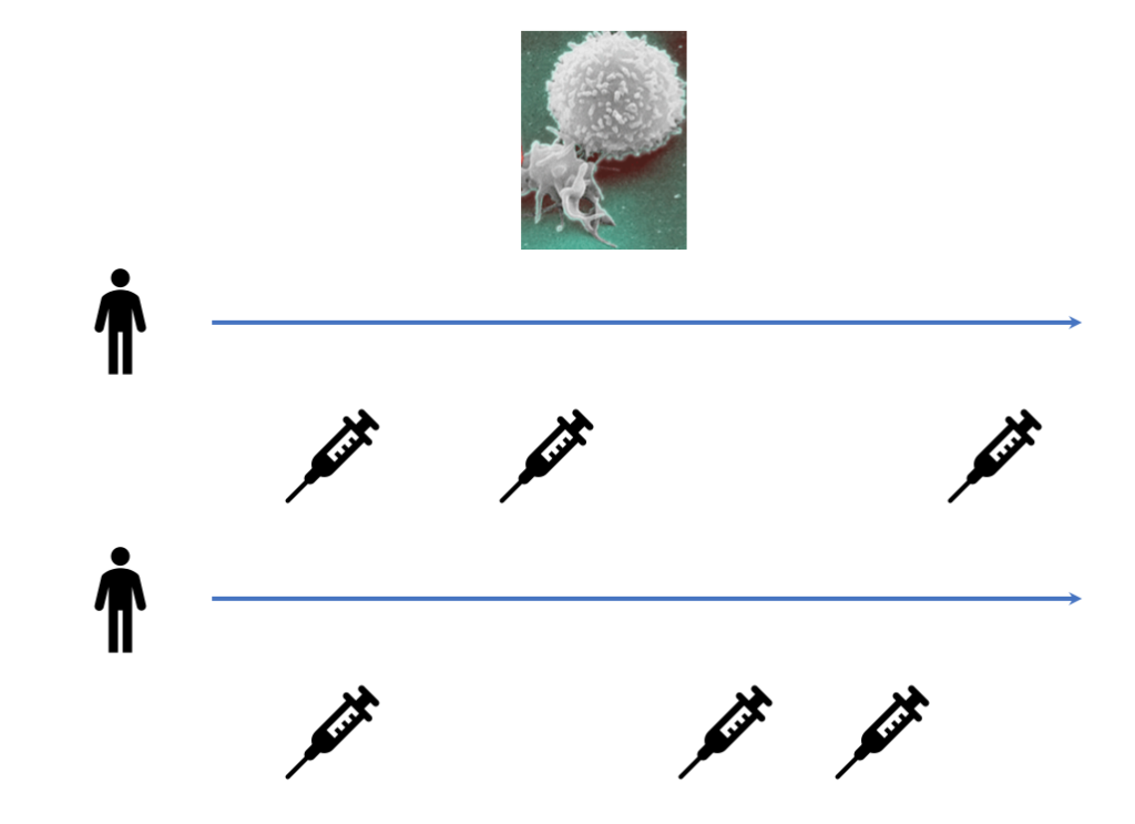
For a static example, say you have a counseling program for smoking and you want to model the effect of some covariates (age, weight, income, etc) on lapse frequency. You have a number of different counselors and each participant is randomized to a different counselor. You expect that both the baseline response and how covariates affect the response varies across counselors. Here the group is the counselor. For a longitudinal example, say you have a number of HIV/AIDS patients and you track their white blood cell counts over time. You want to model the effect of time on white blood cell counts. You expect that the white blood cell count at the start of measurement and the effect of time on the white blood cell count vary between individuals. In this case, the group or cluster is the individual: repeated observations within an individual are correlated.

*Figure 1: we track white blood cell counts over time across several patients, and want to describe how white blood cell counts evolve over time, both within and between patients.*

Intuition

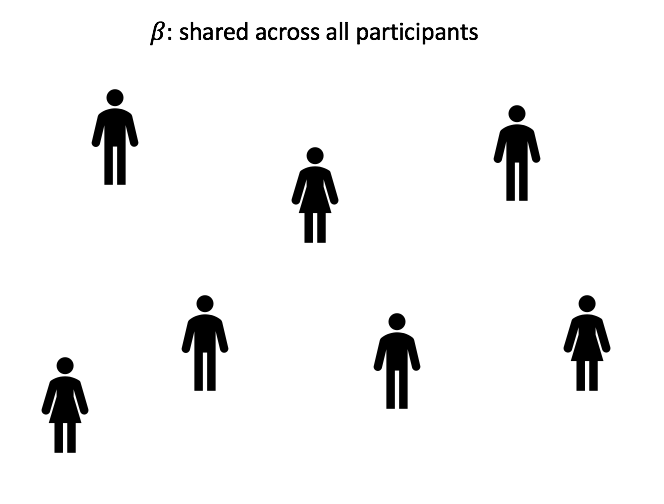
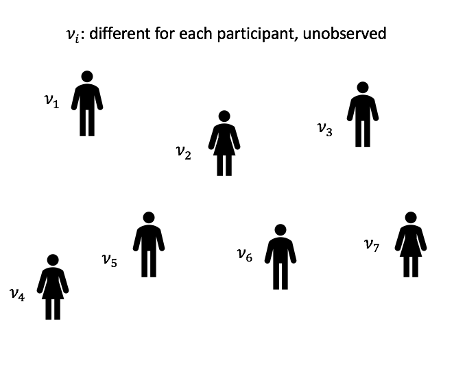
In an LMM for longitudinal data, the observed process is a noisy realization of some linear function of time and possibly other covariates. Further, every individual patient has some deviation from the global behavior. In the HIV/AIDS case, every patient has a different smooth underlying true trajectory, and their observed white blood cell counts are noisy measurements of this true trajectory. We want to first estimate the average trajectory, described by the fixed effects or global parameters $\beta$ . Then we estimate the individual specific deviations from the average trajectory, described by the random effects or latent variables per patient $\nu$ . These definitions of fixed and random effects come from the biostatistics literature: in econometrics fixed and random effects mean something else.

The Model

Scalar Representation

Assume that we have $i=1,2,\cdots,n$ patients or participants in a study, and for each participant, we have $j=1,\cdots,m_i$ observations, where the indexing orders them in time. To start with we look at the case where non-transformed time is the only covariate. Let $y_{ij}$ be the health measurement value for patient $i$ at observation $j$ : this could be the CD4/white blood cell count in AIDS. Then the LMM takes the form

(1)

and

Let $\epsilon_i=(\epsilon_{i1},\cdots,\epsilon_{im_i})^T$ . Then $\epsilon_{i}\sim\mathcal{N}(0,\Sigma_i)$ .
Let $\nu_i=(\nu_{i0},\nu_{i1})^T$ . Then $\nu_i\sim\mathcal{N}(0,G)$
We also assume that all random effect and error vectors are independent from each other. That is, $\epsilon_{1},\epsilon_{2},\cdots,\epsilon_{n},\nu_1,\nu_2,\cdots,\nu_n$ are independent. This is saying that within a patient, random effects are independent of errors, and that we have independence across patients.

Here $(\beta_0,\beta_1)$ are the fixed effects, and $\nu_i$ are the random effects, with $\mathbb{E}(\nu_i)=0$ and $\textrm{Var}(\nu_i)=G$ . The fixed effects can be thought of as the average effects across patients (global parameters in machine learning terminology), while the random effects are the patient specific effects (latent variables per person). The term $\nu_{i0}$ is called the random intercept, and $\nu_{i1}$ is the random slope.

As you may have noticed, we made normality assumptions. In the standard linear regression model with only fixed effects $\beta$ and without random effects, normality assumptions are not necessary to estimate $\beta$ , although they are necessary for confidence intervals when the sample size is small. However, in the mixed model setting, while they are not necessary to fit $\beta$ , they are necessary to derive predictions for $\nu_1,\cdots,\nu_n$ , as we shall see.

Vector and Matrix Representation

We can extend this to a vector-matrix representation along with more features. In the longitudinal case these features may be rich basis functions of time. Let $x_{ij}\in \mathbb{R}^p$ be the covariate vector for fixed effects for patient $i$ at observation $j$ , along with a $1$ in the first position. Let $z_{ij}\in\mathbb{R}^q$ be the same for random effects. In many cases, both of these are simply basis functions of $t_{ij}$ . We can then define

(2)

Here $X$ is the design matrix for for the fixed effects and $Z$ is the design matrix for random effects. Let $y\in \mathbb{R}^m$ be the vector of all observations, where $m=\sum_{i=1}^n m_i$ , and similarly for $\epsilon$ . Further, let

(3)

Then the model is

(4)

where we make the assumptions

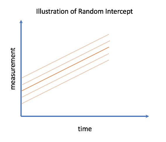
$\left(\begin{array}{c}\epsilon & \nu\end{array}\right)\sim \mathcal{N}\left(\left(\begin{array}{c}0& 0\end{array}\right),\left(\begin{array}{cc} \mathcal{G} & 0\\ 0 & \Sigma\end{array}\right)\right)$

Random Intercept

In a longitudinal setting a random effect which is not associated with a covariate is called the random intercept, and has an important interpretation. It is the deviation from average for the ‘true’ trajectory when they’re first observed. In the HIV/AIDS case, this is how much a patient’s starting health values deviates from average when they enter the study.

Random Slope

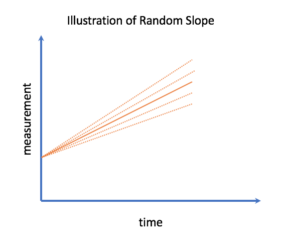
In the case of a single covariate, particularly non-transformed time, we can call the other random effect the random slope. This describes how the rate of evolution of the health process deviates from the average person.

Estimation and Prediction

We first describe how to estimate $\beta$ when both the covariance matrices for random effects $\mathcal{G}$ and for errors $\Sigma$ are known. Then we describe how to predict $\nu$ . In practice, $\mathcal{G}$ and $\Sigma$ are not known, so we then show how to estimate them. Finally, we show how to fit confidence intervals.

Known Covariance Matrix

Expressing the Linear Mixed Model as Gaussian Linear Regression

We can express the model described in part I with fixed and random effects as a Gaussian linear regression problem with only fixed effects (no random effects). Here, however, the covariance matrix between error terms is not only heteroskedastic, but non-diagonal. To see how, consider

(5)

Then since $\left(\begin{array}{c}\epsilon & \nu\end{array}\right)\sim \mathcal{N}\left(\left(\begin{array}{c}0& 0\end{array}\right),\left(\begin{array}{cc} \mathcal{G} & 0\\ 0 & \Sigma\end{array}\right)\right)$ , we have

(6)

With $Y&=X\beta+\epsilon^*$ and $\epsilon^*&\sim\mathcal{N}(0,Z\mathcal{G}Z^T+\Sigma)$ , we have a Gaussian linear regression model. However, the linear regression assumption of independent homoskedastic (equal variance) errors is violated. In particular, for the covariance $Z\mathcal{G}Z^T+\Sigma$ , we can have both non-identical diagonal elements (heteroskedasticity) but also correlation between elements of $\epsilon^*$ . We call this Gaussian linear regression setup the marginal model.

Estimating $\beta$ : Generalized Least Squares

While ordinary least squares is not the best linear unbiased estimator (BLUE) in the presence of correlated heteroskedastic errors, another estimation technique, generalized least squares (GLS), is. Let $V=Z\mathcal{G}Z^T+\Sigma$ be the covariance matrix for $\epsilon^*$ . Then the GLS estimate is given by

(7)

For a derivation of this estimator, see http://halweb.uc3m.es/esp/Personal/personas/durban/esp/web/notes/gls.pdf.

Predicting $\nu$

Since $\nu$ is a random or local latent vector rather than a fixed parameter, we want to predict $\nu$ rather than estimate it. One prediction we can use is $\mathbb{E}(\nu|y)$ . We can calculate this in three steps:

Note that $y$ and $\nu$ are jointly multivariate normal
Compute the covariance between them and get the full joint distribution of the random vector $\left(\begin{array}{c}y \\ \nu\end{array}\right)$ .
Use properties of the multivariate normal to get the conditional expectation

In order to compute the covariance between them, note that

(8)

This gives us that $\left(\begin{array}{c}y \\ \nu\end{array}\right)\sim \mathcal{N}\left(\left(\begin{array}{c}X\beta \\ 0\end{array}\right),\left(\begin{array}{cc}V & Z\mathcal{G} \\ \mathcal{G} Z^T & \mathcal{G}\end{array}\right)\right)$ .

We can then use the conditional expectation for a multivariate normal (see https://stats.stackexchange.com/questions/30588/deriving-the-conditional-distributions-of-a-multivariate-normal-distribution) to obtain

(9)

This is the best linear unbiased predictor (BLUP). To see a proof, see https://dnett.public.iastate.edu/S611/40BLUP.pdf. Next we show what to do when the covariance parameters are unknown.

Unknown Covariance Matrix

Maximizing the Likelihood

One way to estimate $v$ is to maximize the likelihood. Recall that we have the marginal model $Y=X\beta+\epsilon^*$ with $\epsilon^*\sim \mathcal{N}(0,Z\mathcal{G}Z^T+\Sigma)$ , where $Z$ is the design matrix for random effects. Let $V=Z\mathcal{G}Z^T+\Sigma$ . We can assume that both $\mathcal{G}$ and $\Sigma$ are parametrized by variance components $v$ , so that

 (10)

We can then consider the joint log-likelihood of $\beta$ and $v$ , given by

 (11)

however we want to estimate $v$ , so $\beta$ is a nuisance parameter. It is difficult to maximize the joint likelihood directly, but there is an alternate technique for maximizing a joint likelihood in the presence of a nuisance parameter known as the profile likelihood. The idea is to suppose that $v$ is known, and then holding it fixed, derive the maximizing $\tilde{\beta}(v)$ . We can then substitute $\beta$ with $\tilde{\beta}(v)$ in the likelihood, giving us the profile log-likelihood $l_p(v)=l(\tilde{\beta}(v),v)$ , which we maximize with respect to $v$ . The profile likelihood is the joint likelihood with the nuisance parameter expressed as a function of the parameter we want to estimate. As in the above, often this function is the likelihood maximizing expression for the nuisance parameters.

Let $l_v(\beta)$ be the likelihood with $v$ fixed. Overall, we are evaluating the following

 (12)

This gives us the maximum likelihood estimate $\hat{v}_{\textrm{MLE}}$ . For more on the profile log-likelihood, see https://www.stat.tamu.edu/~suhasini/teaching613/chapter3.pdf.

It turns out that the maximum likelihood estimate $\hat{v}_{\textrm{MLE}}$ for $v$ is biased. However, an alternative estimate, the restricted maximum likelihood, is unbiased.

Restricted Maximum Likelihood

The idea for the restricted maximum likelihood (rMEL) for LMM is that instead of maximizing the profile log-likelihood, we maximize the marginal log-likelihood, where we take the joint likelihood and integrate $\beta$ out. Note that this is not the standard intuition for rMEL, but it works for Gaussian LMM. For a more general treatment, see http://people.csail.mit.edu/xiuming/docs/tutorials/reml.pdf.

Let $L(\beta,v)$ be the joint likelihood of $\beta$ and $v$ . Then we want to maximize

 (13)

which is given by (see http://www2.stat.duke.edu/~sayan/Sta613/2017/lec/LMM.pdf for a full derivation)

 (14)

maximizing this gives us the restricted maximum likelihood estimate $\hat{v}_{\textrm{rMEL}}$ , which is unbiased.

Putting it all Together to Estimate $\beta$ and predict $\nu$

Finally, to estimate $\beta$ , we estimate the covariance matrix $V(v)$ from the above, and then estimate $\beta$ as

 (15)

Similarly, to predict $\nu$ , we have

 (16)

Confidence Intervals

Marginal Confidence Intervals for $\hat{\beta}_j$

Since $Y\sim \mathcal{N}(X\beta,V(v))$ and $\hat{\beta}=\left(X^T V^{-1}(\hat{v}X\right)^{-1} X^T V^{-1}(\hat{v})$ , we can derive the covariance matrix for $\hat{\beta}$ .

 (17)

In OLS, the variance of the estimator is a function of the true variance. Here, it is a function of both the true covariance and the estimate of the covariance. Further, in OLS we have an estimator for the error variance that is a scaled $\mathcal{X}^2$ , which allows us to compute exact $t$ marginal confidence intervals under Gaussian errors. We don’t have this here (as far as I know), so we use approximate marginal confidence intervals

 (18)

This will tend to underestimate $\textrm{Var}(\hat{\beta}_j)$ since we didn’t explicitly model the variation in the estimated variance components $\hat{v}$ . However as the sample size grows this will become less of an issue.

Hypothesis Test

We can test the null hypothesis that an individual coefficient is $0$ against the alternative that it is non-zero. That is, test $H_0:\beta_j=0$ versus $H_1:\beta_j\neq 0$ . Let $\hat{\sigma}_j=(X^T V^{-1}(\hat{v})X)^{-1}_{jj}$ . We reject the null $H_0$ if and only if

 (19)

Unfortunately (as far as I know), the finite sample properties of this hypothesis test are not fully understood.