In Survival Analysis, you have three options for modeling the survival function: non-parametric (such as Kaplan-Meier), semi-parametric (Cox regression), and parametric (such as the Weibull distribution). When should you use each? What are their tradeoffs?
Non-Parametric
The most common non-parametric technique for modeling the survival function is the Kaplan-Meier estimate. One way to think about survival analysis is non-negative regression and density estimation for a single random variable (first event time) in the presence of censoring. In line with this, the Kaplan-Meier is a non-parametric density estimate (empirical survival function) in the presence of censoring.
The advantage of this is that it’s very flexible, and model complexity grows with the number of observations. There are two disadvantages: a) it isn’t easy to incorporate covariates, meaning that it’s difficult to describe how individuals differ in their survival functions. The main way to do it is to fit a different model on different subpopulations and compare them. However, as the number of characteristics and values of those characteristics grows, this becomes infeasible. b) the survival functions aren’t smooth. In particular they are piecewise constant. They approach a smooth estimator as the sample size grows, but for small samples they are far from smooth and can have unrealistic properties. For instance the death probability may ‘jumps’ by a huge amount over a small period of time. Further, if you don’t have any death observations in the interval [0,t), then it will assign survival probability 1 to that period, which may not be desirable or realistic. There are ways to smooth the survival function (kernel smoothing), but the interpretation of the smoothing can be a bit tricky.
Let’s look at an example. We use the ovarian dataset from the R package ‘survival.’ We borrow some code from this tutorial in order to pre-process the data and make this plot. The data has death or censoring times for ovarian cancer patients over a period of approximately 1200 days. It also has the treatment rx (1 or 2), a diagnosis on regression of tumors, and patient performance on an ECOG criteria. Here is a plot of two Kaplan Meier fits according to treatment: this plot is generated by the following code which we lifted directly from the previous tutorial (which also contains other code).
<pre class="wp-block-syntaxhighlighter-code">library(survival)
library(survminer)
library(dplyr)
# Dichotomize age and change data labels
ovarian<img src="https://boostedml.com/wp-content/ql-cache/quicklatex.com-9c6809fb2b76e4b5e064fd741b1ed3a5_l3.png" class="ql-img-inline-formula quicklatex-auto-format" alt="rx <- factor(ovarian" title="Rendered by QuickLaTeX.com" height="19" width="176" style="vertical-align: -5px;"/>rx,
levels = c("1", "2"),
labels = c("A", "B"))
ovarian<img src="https://boostedml.com/wp-content/ql-cache/quicklatex.com-f3932b69f0f5cccd5ab8ee61a54f88f8_l3.png" class="ql-img-inline-formula quicklatex-auto-format" alt="resid.ds <- factor(ovarian" title="Rendered by QuickLaTeX.com" height="19" width="220" style="vertical-align: -5px;"/>resid.ds,
levels = c("1", "2"),
labels = c("no", "yes"))
ovarian<img src="https://boostedml.com/wp-content/ql-cache/quicklatex.com-7e67a0ec867712bc8e822f0c95d00295_l3.png" class="ql-img-inline-formula quicklatex-auto-format" alt="ecog.ps <- factor(ovarian" title="Rendered by QuickLaTeX.com" height="19" width="213" style="vertical-align: -5px;"/>ecog.ps,
levels = c("1", "2"),
labels = c("good", "bad"))
surv_object <- Surv(time = ovarian<img src="https://boostedml.com/wp-content/ql-cache/quicklatex.com-fbf30b4e777f55822030ebcc91818d81_l3.png" class="ql-img-inline-formula quicklatex-auto-format" alt="futime, event = ovarian" title="Rendered by QuickLaTeX.com" height="16" width="193" style="vertical-align: -4px;"/>fustat)
fit1 <- survfit(surv_object ~ rx, data = ovarian)
ggsurvplot(fit1, data = ovarian, pval = TRUE)
</pre>
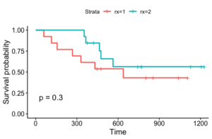
This plot has some of the issues we mentioned. Firstly, the survival probabilities ‘jump.’ Secondly, for rx=2, we see that for the first 350 or so days, no one died, and thus we see a survival probability of 1. It can be dangerous to presume that this is close to the true survival probability, particularly if the data size for that group is small. Finally, if we want to incorporate the tumor regression diagnosis or patient performance in addition to treatment, we’ll need to fit many different models, one for each possible combination of values of covariates.
Semi-Parametric
The most well-known semi-parametric technique is Cox regression. This addresses the problem of incorporating covariates. It decomposes the hazard or instantaneous risk into a non-parametric baseline, shared across all patients, and a relative risk, which describes how individual covariates affect risk.
(1) 
This allows for a time-varying baseline risk, like in the Kaplan Meier model, while allowing patients to have different survival functions within the same fitted model. Again though, the survival function is not smooth. Further, we now have to satisfy the parametric assumptions for the effects of covariates on the hazard. For the Cox proportional hazards, it is a log-linear assumption (proportional hazards). For other models such as Aalen’s additive model, it may be a linear assumption.
We can fit a Cox model, regressing on rx as follows
fitcox <- coxph(Surv(futime, fustat) ~ rx, data = ovarian)
fitcox

Call:
coxph(formula = Surv(futime, fustat) ~ rx, data = ovarian)

       coef exp(coef) se(coef)      z    p
rxB -0.5964    0.5508   0.5870 -1.016 0.31

Likelihood ratio test=1.05  on 1 df, p=0.3052
n= 26, number of events= 12
Note that given the non-parametric plot we previously showed, a proportional hazards model is actually not a great fit to this data, as under proportional hazards we should see that the survival curves have similar basic shape but diverge. We can test the proportional hazards assumption for this regression model.
testcox<-cox.zph(fitcox)
testcox

chisq df   p
rx      2.68  1 0.1
GLOBAL  2.68  1 0.1

ggcoxzph(testcox)
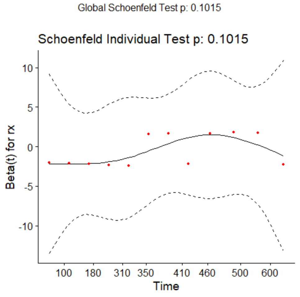
Here we would like the slope to be  . There seems to be some violations although they are not quite significant.
Parametric
One can also assume that the survival function follows a parametric distribution. For instance, one can assume an exponential distribution (constant hazard) or a Weibull distribution (time-varying hazard). There are now two benefits. The first is that if you choose an absolutely continuous distribution, the survival function is now smooth. The second is that choosing a parametric survival function constrains the model flexibility, which may be good when you don’t have a lot of data and your choice of parametric model is appropriate. Unlike applying a smoothing technique after an initial estimation of the survival function, for these parametric models we tend to have good intuition for how they behave. Further, like in Cox regression, it’s easy to incorporate covariates into the model and inference procedure.
The downside is that one needs the parametric model to actually be a good description of your data. This may or may not be true, and one needs to test it, either by formal hypothesis testing or visualization procedures.
One example is a parametric proportional hazards model. This takes the same form
(2)
but in this case the baseline hazard  is now parametric. We can fit this as follows:
library(eha)

fitparam <- phreg(Surv(futime, fustat) ~ rx, data = ovarian)
fitparam

Call:
phreg(formula = Surv(futime, fustat) ~ rx, data = ovarian)

Covariate          W.mean      Coef Exp(Coef)  se(Coef)    Wald p
rx
               A    0.431     0         1           (reference)
               B    0.569    -0.631     0.532     0.587     0.282

log(scale)                    6.825               0.344     0.000
log(shape)                    0.121               0.251     0.629

Events                    12
Total time at risk         15588
Max. log. likelihood      -97.364
LR test statistic         1.18
Degrees of freedom        1
Overall p-value           0.277458
Question to Ask
When deciding which type of model to fit. Ask yourself the following questions:
- Do you need covariates? Lean towards parametric or semi-parametric. Make sure assumptions are satisfied.
- Do you need your survival function to be smooth? Lean towards parametric, or apply a smoothing technique.
- Does your data appear to follow a parametric distribution? Lean towards parametric if it does. Otherwise semi-parametric or non-parametric.